插值、拟合、积分

[TOC]

Overview

• 插值：求过已知有限个数据点的近似函数。

• 拟合：已知有限个数据点，求近似函数，不要求过已知数据点，只要求在某种意义下它在这些点上的总偏差最小。

插值和拟合都是要根据一组数据构造一个函数作为近似，由于近似的要求不同，二者的数学方法上是完全不同的。而面对一个实际问题，究竟应该用插值还是拟合，有时容易确定，有时则并不明显。

插值

Comparison of 1D and 2D Interpolations

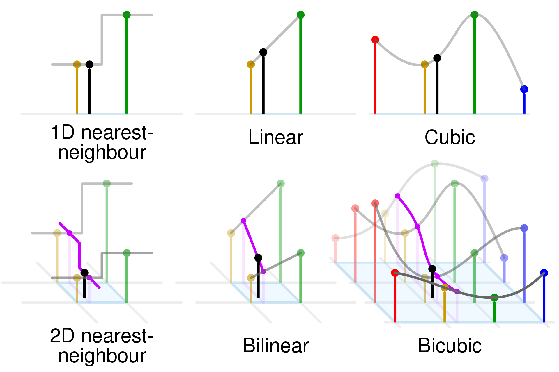
最近邻插值

1D Nearest Interpolation

2D Nearest Interpolation

\[ \mathbf{I}_\mathrm{dst}(i, j) = \mathbf{I}_\mathrm{src}(u^{\prime}, v^{\prime}) = \mathbf{I}_\mathrm{src}(u, v) \]

with

\[ (i, j) \Rightarrow (u^{\prime}, v^{\prime}) \Rightarrow \begin{cases} u = \text{round}(u^{\prime}) \\ v = \text{round}(v^{\prime}) \end{cases} \]

case INTERPOLATION_NEAREST: {
    int lx = static_cast<int>(std::round(x));
    int ly = static_cast<int>(std::round(y));
    result = (this)(ly, lx);
}

线性插值

Linear Interpolation (Lerp)

Bilinear Interpolation

\[ \mathbf{I}_\mathrm{dst}(i, j) = \mathbf{I}_\mathrm{src}(u^{\prime}, v^{\prime}) = \mathbf{I}_\mathrm{src}(u+\alpha, v+\beta) \]

with

\[ (i, j) \Rightarrow (u^{\prime}, v^{\prime}) \Rightarrow \begin{cases} u = \text{floor}(u^{\prime}) = \lfloor u^{\prime} \rfloor \\ v = \text{floor}(v^{\prime}) = \lfloor v^{\prime} \rfloor \end{cases} \Rightarrow \begin{cases} \alpha = u^{\prime} - u \\ \beta = v^{\prime} - v \end{cases} \]

令

\[ \begin{aligned} f_{00} &= f(u, v) \\ f_{01} &= f(u, v + 1) \\ f_{10} &= f(u + 1, v) \\ f_{11} &= f(u + 1, v + 1) \end{aligned} \]

（1） V方向线性插值

\[ \begin{cases} f(u, & v+\beta) = (f_{01} - f_{00}) \beta + f_{00} \\ f(u+1, & v+\beta) = (f_{11} - f_{10}) \beta + f_{10} \end{cases} \]

（2） U方向线性插值

\[ f(u+\alpha, v+\beta) = [f(u+1, v+\beta) - f(u, v+\beta)]\alpha + f(u, v+\beta) \]

（3）最终

\[ f(u+\alpha, v+\beta) = [(1-\alpha)(1-\beta)]f_{00} + \beta (1-\alpha) f_{01} + \alpha (1-\beta) f_{10} + \alpha \beta f_{11} \]

case INTERPOLATION_BILINEAR: {
    const int lx = std::floor(x);
    const int ly = std::floor(y);

    T f00 = (this)(ly, lx);
    T f01 = (this)(ly + 1, lx);
    T f10 = (this)(ly, lx + 1);
    T f11 = (this)(ly + 1, lx + 1);

    double alpha = x - lx;
    double beta  = y - ly;

    result =
      (1 - beta) * ((1 - alpha) * f00 + alpha * f10) +
      beta * ((1 - alpha) * f01 + alpha * f11);
}

Spherical Linear Interpolation (Slerp)

• Ref: ESKF 2.7
• https://splines.readthedocs.io/en/latest/rotation/slerp.html

\[ \mathbf{q}(t)=\mathbf{q}_{0} \frac{\sin ((1-t) \Delta \theta)}{\sin (\Delta \theta)}+\mathbf{q}_{1} \frac{\sin (t \Delta \theta)}{\sin (\Delta \theta)} \]

Quaterniond slerp(double t, Quaterniond &q1, Quaterniond &q2) {
    Quaterniond q_slerp;
    float cos_q1q2 = q1.w() * q2.w() + q1.x() * q2.x() + q1.y() * q2.y() + q1.z() * q2.z();

    if (cos_q1q2 < 0.0f) {
        q1.w() = -1 * q1.w();
        q1.x() = -1 * q1.x();
        q1.y() = -1 * q1.y();
        q1.z() = -1 * q1.z();
        //cos_q1q2=-1*cos_q1q2;
        cos_q1q2 = q1.w() * q2.w() + q1.x() * q2.x() + q1.y() * q2.y() + q1.z() * q2.z();
    }

    float k1, k2;

    if (cos_q1q2 > 0.9995f) {
        k1 = 1.0f - t;
        k2 = t;
    } else {
        float sin_q1q2 = sqrt(1.0f - cos_q1q2 * cos_q1q2);
        float q1q2 = atan2(sin_q1q2, cos_q1q2);
        k1 = sin((1.0f - t) * q1q2) / sin_q1q2;
        k2 = sin(t * q1q2) / sin_q1q2;
    }

    q_slerp.w() = k1 * q1.w() + k2 * q2.w();
    q_slerp.x() = k1 * q1.x() + k2 * q2.x();
    q_slerp.y() = k1 * q1.y() + k2 * q2.y();
    q_slerp.z() = k1 * q1.z() + k2 * q2.z();

    return q_slerp;
}

Slerp v.s. Nlerp

• Nlerp: Normalized Linear Interpolation

样条插值 (Spline)

Bezier Curve

Cubic Spline Interpolation

B-Spline

• B-Spline for SLAM

积分

Runge-Kutta numerical integration methods

The Euler method

\[ \mathbf{x}_{n+1}=\mathbf{x}_{n}+\Delta t \cdot k_1 \]

where

\[ k_1 = f\left(t_{n}, \mathbf{x}_{n}\right) \]

The midpoint method

\[ \mathbf{x}_{n+1} = \mathbf{x}_{n} + \Delta t \cdot k_2 \]

where

\[ k_2 = f\left(t_{n}+\frac{1}{2} \Delta t, \mathbf{x}_{n} + \frac{\Delta t}{2} \cdot k_1\right) \]

The RK4 method

\[ \mathbf{x}_{n+1}=\mathbf{x}_{n}+\frac{\Delta t}{6}\left(k_{1}+2 k_{2}+2 k_{3}+k_{4}\right) \]

where

\[ \begin{aligned} k_{1} &=f\left(t_{n}, \mathbf{x}_{n}\right) \\ k_{2} &=f\left(t_{n}+\frac{1}{2} \Delta t, \mathbf{x}_{n}+\frac{\Delta t}{2} k_{1}\right) \\ k_{3} &=f\left(t_{n}+\frac{1}{2} \Delta t, \mathbf{x}_{n}+\frac{\Delta t}{2} k_{2}\right) \\ k_{4} &=f\left(t_{n}+\Delta t, \mathbf{x}_{n}+\Delta t \cdot k_{3}\right) \end{aligned} \]

General Runge-Kutta method

\[ \mathbf{x}_{n+1}=\mathbf{x}_{n}+\Delta t \sum_{i=1}^{s} b_{i} k_{i} \]

where

\[ k_{i}=f\left(t_{n}+\Delta t \cdot c_{i}, \mathbf{x}_{n}+\Delta t \sum_{j=1}^{s} a_{i j} k_{j}\right) \]