3D欧式变换之旋转ABC

本文最后更新于：May 7, 2023 pm

Overview

旋转转换
- Maths - Rotation conversions
- ptam_cg/src/Tools.cc

旋转表示

旋转矩阵 (Rotation Matrix)

\[ \mathbf{R} = \begin{bmatrix} r_{11} & r_{12} & r_{13} \\ r_{21} & r_{22} & r_{23} \\ r_{31} & r_{32} & r_{33} \end{bmatrix} \in \mathbb{R}^{3 \times 3}, \quad s.t. \quad \mathbf{RR}^T = \mathbf{I}, \det(\mathbf{R}) = 1 \]

旋转矩阵归一化

我们通过某些计算得出的“旋转矩阵”可能不符合旋转矩阵的条件，需要对其归一化

// ref ORB-SLAM3
cv::Mat NormalizeRotation(const cv::Mat &R)
{
    cv::Mat U,w,Vt;
    cv::SVDecomp(R,w,U,Vt,cv::SVD::FULL_UV);
    return U*Vt;
}

旋转向量/轴角 (Rotation Vector)

\[ \boldsymbol{\phi} = \mathbf{u} \theta = \log(\mathbf{R})^{\vee} \in \mathbb{R}^3 \]

旋转轴：矩阵 \(\mathbf{R}\) 特征值1对应的特征向量（单位矢量） \[ \mathbf{u} = \frac{\boldsymbol{\phi}}{||\boldsymbol{\phi}||} \in \mathbb{R}^3 \]
旋转角 \[ \theta = ||\boldsymbol{\phi}|| = \arccos \left(\frac{tr(\mathbf{R})-1}{2} \right) \in \mathbb{R} \]

旋转向量与旋转矩阵的转换，罗德里格斯公式 ^[2]

\[ \mathbf{R} = \cos \theta \mathbf{I} + (1-\cos \theta) \mathbf{uu}^T + \sin \theta \mathbf{u}^{\wedge} \]

Rotation/Unit Quarternion ^[1]

Lie Group & Lie Algebra \(SO(3)\) ^[1]

Euler Angle

旋转矩阵可以可以分解为绕各自轴对应旋转矩阵的乘积：

\[ \mathbf{R} = \mathbf{R}_1 \mathbf{R}_2 \mathbf{R}_3 \]

根据绕轴的不同，欧拉角共分为两大类，共12种，如下图（基于 右手系）所示：

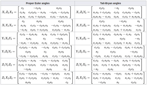
以上不同旋转轴合成的旋转矩阵，每一种都可以看成 同一旋转矩阵的两种不同物理变换：

绕 固定轴 旋转
绕动轴旋转

以 \(Z_1Y_2X_3\) 进行为例，旋转矩阵表示为 \(\mathbf{R} = \mathbf{R}_z \mathbf{R}_y \mathbf{R}_x\)，说明：

绕 固定轴 旋转：以初始坐标系作为固定坐标系，分别先后绕固定坐标系的X、Y、Z轴 旋转；
绕动轴旋转：先绕 初始Z轴 旋转，再绕 变换后的Y轴 旋转，最后绕 变换后的X轴 旋转

即绕 固定坐标轴的XYZ 和 绕运动坐标轴的ZYX 的旋转矩阵是一样的。

我们经常用的欧拉角一般就是 \(Z_1Y_2X_3\) 轴序的 yaw-pitch-roll，如下图所示：

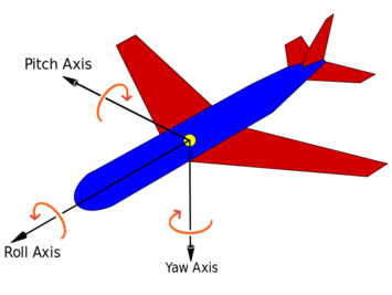
对应的旋转矩阵为

\[ \mathbf{R} = \mathbf{R}_z \mathbf{R}_y \mathbf{R}_x = \mathbf{R}(\theta_{yaw}) \mathbf{R}(\theta_{pitch}) \mathbf{R}(\theta_{roll}) \]

其逆矩阵为：

\[ \begin{aligned} \mathbf{R}^{-1} &= (\mathbf{R}_z \mathbf{R}_y \mathbf{R}_x)^{-1} \\ &= \mathbf{R}_x^{-1} \mathbf{R}_y^{-1} \mathbf{R}_z^{-1} \\ &= \mathbf{R}(-\theta_{roll}) \mathbf{R}(-\theta_{pitch}) \mathbf{R}(-\theta_{yaw}) \end{aligned} \]

上面 \(\mathbf{R}_x \mathbf{R}_y \mathbf{R}_z\) 以 Cosine Matrix 的形式表示为（右手系）：

\[ \mathbf{R}_x(\theta) = \begin{bmatrix} 1 & 0 & 0 \\ 0 & \cos(\theta) & -\sin(\theta) \\ 0 & \sin(\theta) & \cos(\theta) \end{bmatrix} \]

\[ \mathbf{R}_y(\theta) = \begin{bmatrix} \cos(\theta) & 0 & \sin(\theta) \\ 0 & 1 & 0 \\ -\sin(\theta) & 0 & \cos(\theta) \end{bmatrix} \]

\[ \mathbf{R}_z(\theta) = \begin{bmatrix} \cos(\theta) & -\sin(\theta) & 0 \\ \sin(\theta) & \cos(\theta) & 0 \\ 0 & 0 & 1 \end{bmatrix} \]

Compare ^[4]

四元数和旋转矩阵、旋转向量相比究竟有何优势？ ^[5] ^[6]

平滑插值
内存和运算速度更优
- 内存上，一个四元数只占四个浮点数
- 在四元数相乘时可以直接在这四个数上进行加减乘的基本运算，比旋转向量转换成旋转矩阵相乘后再转换回旋转向量要高效得多（Rodrigues 变换还涉及除法和三角函数等高级运算）。这些在嵌入式平台上是不小的优势
浮点数运算总是会有误差的，运算越多，误差累计越多，所以理论上四元数相乘也有精度上的优势

旋转方式

active rotation: rotating vectors
passive rotation: rotating frames

旋转小量

若小旋转向量 \(\Delta \boldsymbol{\phi}\)，则旋转小量一阶近似

\[ \Delta \mathbf{R} = \exp({\Delta \boldsymbol{\phi}}^\wedge) \approx \mathbf{I} + {\Delta \boldsymbol{\phi}}^\wedge \]

\[ \Delta \mathbf{q} \approx \begin{bmatrix} 1 \\ \frac{1}{2} \Delta \boldsymbol{\phi} \end{bmatrix} \]

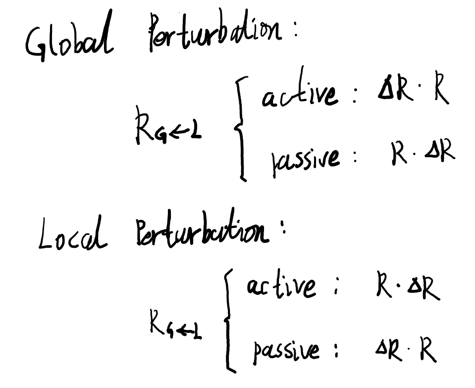
旋转扰动

Local Perturbation
Global Perturbation

旋转更新

\[ \boxplus(x, \Delta) \]

对于 Manifold空间的状态 \(x\)，因不能直接相加，取其 Tangent空间小量，再将其映射回 Manifold空间。

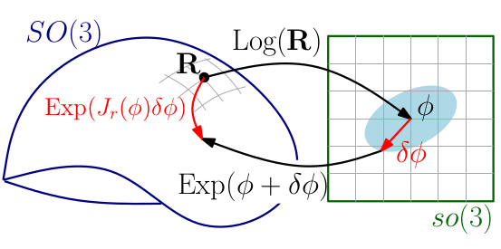
即（BCH公式）

\[ \exp((\theta + \delta \theta)^{\wedge}) \approx \exp({\theta}^{\wedge}) \cdot \exp((J_r \delta \theta)^{\wedge}) = R \cdot \exp((J_r \delta \theta)^{\wedge}) \]

而实际上，已知状态旋转向量 \(\theta\)，其对应旋转矩阵 \(R(\theta)\)，旋转小量 \(\Delta R(\delta \theta)\) 或 \(\Delta q(\delta \theta)\) 对其进行更新，VINS-Mono、MSCKF、ORB-SLAM等开源代码中都是如下直接右乘

\[ \mathbf{R} \leftarrow \mathbf{R} \cdot \Delta \mathbf{R} \]

\[ \mathbf{q} \leftarrow \mathbf{q} \otimes \Delta \mathbf{q} \]

四元数形式

右乘更新（MSCKF、VINS-Mono）

\[ q^\prime = q \cdot \delta q, \quad \text{normalize} \; q^\prime, \quad s.t. \quad \delta q = \begin{bmatrix} 1 \\ \frac{1}{2} \delta \theta \end{bmatrix} \]

而实际上

\[ q(\theta + \delta \theta) = \exp(\frac{\theta + \delta \theta}{2}) \]

OKVIS中左乘

\[ q^\prime = \delta q \cdot q \]

// apply small update:
template<typename Derived_delta>
inline bool Transformation::oplus(
    const Eigen::MatrixBase<Derived_delta> & delta) {
  r_ += delta.template head<3>();
  Eigen::Vector4d dq;
  double halfnorm = 0.5 * delta.template tail<3>().norm();
  dq.template head<3>() = sinc(halfnorm) * 0.5 * delta.template tail<3>();
  dq[3] = cos(halfnorm);
  q_ = (Eigen::Quaterniond(dq) * q_);
  return true;
}

李群李代数形式

g2o中更新，左乘

\[ \exp({\delta \theta}^{\wedge}) \cdot R \]

/**
 * \brief SE3 Vertex parameterized internally with a transformation matrix
 and externally with its exponential map
 */
class  VertexSE3Expmap : public BaseVertex<6, SE3Quat>{
public:
  EIGEN_MAKE_ALIGNED_OPERATOR_NEW

  VertexSE3Expmap();

  bool read(std::istream& is);

  bool write(std::ostream& os) const;

  virtual void setToOriginImpl() {
    _estimate = SE3Quat();
  }

  virtual void oplusImpl(const double* update_)  {
    Eigen::Map<const Vector6d> update(update_);
    setEstimate(SE3Quat::exp(update)*estimate());
  }
};

ORB-SLAM3中更新，右乘

\[ R \cdot \exp({\delta \theta}^{\wedge}) \]

void ImuCamPose::Update(const double *pu)
{
    Eigen::Vector3d ur, ut;
    ur << pu[0], pu[1], pu[2];
    ut << pu[3], pu[4], pu[5];

    // Update body pose
    twb += Rwb*ut;
    Rwb = Rwb*ExpSO3(ur);

    // Normalize rotation after 5 updates
    its++;
    if(its>=3)
    {
        NormalizeRotation(Rwb);
        its=0;
    }
}

旋转残差

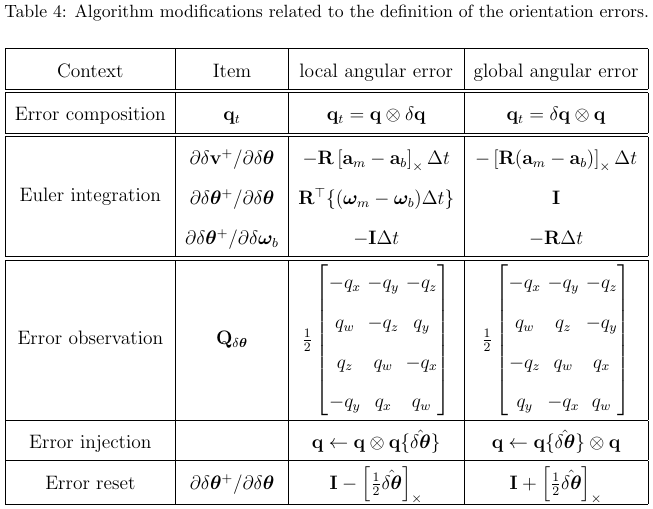
global angular error

\[ \Delta R = R_1 \cdot R_2^{-1} \]

local angular error (VINS-Mono & ORB-SLAM3)

\[ \Delta R = R_2^{-1} \cdot R_1 \]

不能像下面这样直接减：

\[ \delta \theta = \theta_1 - \theta_2 \longrightarrow \Delta R = R_1 \cdot R_2^{-1} \]

（1）四元数形式（VINS-Mono）

\[ \delta \theta = 2 \left[ q(\Delta R) \right]_{\mathtt{vec}} / q_w \]

（2）李群李代数形式

\[ \delta \theta = [\ln(\Delta R)]^{\vee} \]

g2o中，两个位姿为顶点时的残差:

void EdgeSE3Expmap::computeError() {
  const VertexSE3Expmap* v1 = static_cast<const VertexSE3Expmap*>(_vertices[0]);
  const VertexSE3Expmap* v2 = static_cast<const VertexSE3Expmap*>(_vertices[1]);

  SE3Quat C(_measurement);
  SE3Quat error_ = v2->estimate().inverse() * C * v1->estimate();
  _error = error_.log();
}

旋转导数 (雅克比矩阵)

对时间求导

若角速度为 \(\boldsymbol{\omega}\)，那么旋转的时间导数为

\[ \dot{\mathbf{q}} = \mathbf{q} \otimes \begin{bmatrix} 0 \\ \frac{1}{2} \boldsymbol{\omega} \end{bmatrix} = \frac{1}{2} \mathbf{q} \otimes \begin{bmatrix} 0 \\ \boldsymbol{\omega} \end{bmatrix} \]

\[ \dot{\mathbf{R}}=\mathbf{R} \boldsymbol{\omega}^{\wedge} \]

对旋转求导

李代数求导

用李代数表示位姿，然后根据李代数加法来对李代数求导

\[ \begin{aligned} \frac{\partial(\mathbf{R} \mathbf{p})}{\partial \phi} &= \frac{\partial\left(\exp \left(\boldsymbol{\phi}^{\wedge}\right) \mathbf{p}\right)}{\partial \boldsymbol{\phi}} \\ &=\lim _{\delta \phi \rightarrow 0} \frac{\exp \left((\boldsymbol{\phi}+\delta \boldsymbol{\phi})^{\wedge}\right) \mathbf{p}-\exp \left(\boldsymbol{\phi}^{\wedge}\right) \mathbf{p}}{\delta \boldsymbol{\phi}} \\ &=\lim _{\delta \boldsymbol{\phi} \rightarrow 0} \frac{\exp \left(\left(\boldsymbol{J}_{l} \delta \boldsymbol{\phi}\right)^{\wedge}\right) \exp \left(\boldsymbol{\phi}^{\wedge}\right) \mathbf{p}-\exp \left(\boldsymbol{\phi}^{\wedge}\right) \mathbf{p}}{\delta \boldsymbol{\phi}} \\ & \approx \lim _{\delta \boldsymbol{\phi} \rightarrow 0} \frac{\left(\boldsymbol{I}+\left(\boldsymbol{J}_{l} \delta \boldsymbol{\phi}\right)^{\wedge}\right) \exp \left(\boldsymbol{\phi}^{\wedge}\right) \mathbf{p}-\exp \left(\boldsymbol{\phi}^{\wedge}\right) \mathbf{p}}{\delta \boldsymbol{\phi}} \\ &=\lim _{\delta \boldsymbol{\phi} \rightarrow 0} \frac{\left(\boldsymbol{J}_{l} \delta \boldsymbol{\phi}\right)^{\wedge} \exp \left(\boldsymbol{\phi}^{\wedge}\right) \mathbf{p}}{\delta \boldsymbol{\phi}} \\ &=\lim _{\delta \boldsymbol{\phi} \rightarrow 0} \frac{-\left(\exp \left(\boldsymbol{\phi}^{\wedge}\right) \mathbf{p}\right)^{\wedge} \boldsymbol{J}_{l} \delta \boldsymbol{\phi}}{\delta \boldsymbol{\phi}}=-(\mathbf{R} \mathbf{p})^{\wedge} \boldsymbol{J}_{l} \end{aligned} \]

其中，\(\mathbf{J}_l\) 为 \(SO(3)\) 的左雅克比矩阵，其定义为

\[ \boldsymbol{J}_{l}=\boldsymbol{J}=\frac{\sin \theta}{\theta} \boldsymbol{I}+\left(1-\frac{\sin \theta}{\theta}\right) \boldsymbol{a} \boldsymbol{a}^{T}+\frac{1-\cos \theta}{\theta} \boldsymbol{a}^{\wedge} \]

w.r.t Error State

\[ \frac{\partial f(x)}{\partial \delta x} = \frac{\partial f(x)}{\partial x} \cdot \frac{\partial x}{\partial \delta x} \]

对于欧式空间

\[ \frac{\partial x}{\partial \delta x} = I \]

对于流行空间，例如旋转 \(q\)

扰动方式

Note: 本质是 Local 或 Global 扰动

对李群左乘或者右乘微小扰动量，然后对该扰动求导，成为左扰动和右扰动模型，这种方式 省去了计算雅克比，所以使用更为常见

\[ \begin{aligned} \frac{\partial(\mathbf{R} \mathbf{p})}{\partial \boldsymbol{\phi}} &=\lim _{\boldsymbol{\varphi} \rightarrow 0} \frac{\exp \left(\boldsymbol{\varphi}^{\wedge}\right) \exp \left(\boldsymbol{\phi}^{\wedge}\right) \mathbf{p}-\exp \left(\boldsymbol{\phi}^{\wedge}\right) \mathbf{p}}{\varphi} \\ & \approx \lim _{\varphi \rightarrow 0} \frac{\left(I+\boldsymbol{\varphi}^{\wedge}\right) \exp \left(\boldsymbol{\phi}^{\wedge}\right) \mathbf{p}-\exp \left(\boldsymbol{\phi}^{\wedge}\right) \mathbf{p}}{\varphi} \\ &=\lim _{\boldsymbol{\varphi} \rightarrow 0} \frac{\boldsymbol{\varphi}^{\wedge} \mathbf{R} \mathbf{p}}{\varphi} \\ &=\lim _{\varphi \rightarrow 0} \frac{-(\mathbf{R} \mathbf{p})^{\wedge} \boldsymbol{\varphi}}{\varphi} \\ &=-(\mathbf{R} \mathbf{p})^{\wedge} \end{aligned} \]

\[ \begin{aligned} \frac{\partial{(\mathbf{R}^{-1} \mathbf{p})}}{\partial{\boldsymbol{\phi}}} &= \lim_{\varphi \rightarrow 0} \frac{(\mathbf{R}\exp(\varphi^{\wedge}))^{-1} \mathbf{p} - \mathbf{R}^{-1} \mathbf{p}} {\varphi} \\ &= \lim_{\varphi \rightarrow 0} \frac{\exp(-\varphi^{\wedge}) \mathbf{R}^{-1} \mathbf{p} - \mathbf{R}^{-1} \mathbf{p}} {\varphi} \\ &\approx \lim_{\varphi \rightarrow 0} \frac{(\mathbf{I}-\varphi^{\wedge}) \mathbf{R}^{-1} \mathbf{p} - \mathbf{R}^{-1} \mathbf{p}} {\varphi} \\ &= \lim_{\varphi \rightarrow 0} \frac{-\varphi^{\wedge} \mathbf{R}^{-1} \mathbf{p}} {\varphi} \\ &= \lim_{\varphi \rightarrow 0} \frac{(\mathbf{R}^{-1}\mathbf{p})^{\wedge} \varphi} {\varphi} \\ &= (\mathbf{R}^{-1}\mathbf{p})^{\wedge} \end{aligned} \]

\[ \begin{aligned} \frac{\partial \ln(\mathbf{R}_1 \mathbf{R}_2^{-1})^{\vee}}{\partial \boldsymbol{\phi}_2} &= \lim_{\varphi \rightarrow 0} \frac{\ln(\mathbf{R}_1 (\mathbf{R}_2 \exp(\varphi^{\wedge}))^{-1})^{\vee} - \ln(\mathbf{R}_1 \mathbf{R}_2^{-1})^{\vee}} {\varphi} \\ &= \lim_{\varphi \rightarrow 0} \frac{\ln(\mathbf{R}_1 \exp(-\varphi^{\wedge}) \mathbf{R}_2^{-1})^{\vee} - \ln(\mathbf{R}_1 \mathbf{R}_2^{-1})^{\vee}} {\varphi} \\ &= \lim_{\varphi \rightarrow 0} \frac{\ln(\mathbf{R}_1 \mathbf{R}_2^{-1} \exp((-\mathbf{R}_2 \varphi)^{\wedge}))^{\vee} - \ln(\mathbf{R}_1\mathbf{R}_2^{-1})^{\vee}} {\varphi} \\ &\approx \lim_{\varphi \rightarrow 0} \frac{\ln(\mathbf{R}_1\mathbf{R}_2^{-1})^{\vee} + \mathbf{J}_r^{-1} (-\mathbf{R}_2 \varphi) - \ln(\mathbf{R}_1\mathbf{R}_2^{-1})^{\vee}} {\varphi} \\ &= -\mathbf{J}_r^{-1} \mathbf{R}_2 \end{aligned} \]

对于矩阵A和B，\(\exp(A)\exp(B) \neq \exp(A+B)\)，错误示例：

\[ r = \ln(R_1 \cdot R_2^T)^\vee = \ln \left[ \exp({\theta}_1^{\wedge}) \cdot \exp(-{\theta}_2^{\wedge}) \right]^\vee = {\theta}_1 - {\theta}_2 \]

四元数形式

\[ r = \delta \theta = 2 \left[ q_1 \otimes q_2^{-1} \right]_{xyz} = 2 \left[ q_1 \otimes q_2^{*} \right]_{xyz} \]

\[ \begin{aligned} \frac{\partial r}{\partial \delta {\theta}_2} &= \frac{\partial 2 \left[ q_1 \otimes q_2^{*} \right]_{xyz}}{\partial \delta {\theta}_2} \\ &= \frac {\partial 2 \left[ q_1 \otimes \left[ q_2 \otimes \delta q_2 \right]^{*} \right]_{xyz}} {\partial \delta {\theta}_2} \\ &= -2 \begin{bmatrix} 0 & I \end{bmatrix}_{3 \times 4} \cdot \frac{\partial \left[ q_2 \otimes \delta q_2 \otimes q_1^* \right]} {\partial \delta {\theta}_2} \\ &= -2 \begin{bmatrix} 0 & I \end{bmatrix}_{3 \times 4} \cdot \frac{\partial \left[ L(q_2) \cdot R(q_1^*) \cdot \delta q_2 \right]} {\partial \delta q_2} \cdot \frac{\partial \delta q_2} {\partial {\theta}_2} \\ &= -2 \begin{bmatrix} 0 & I \end{bmatrix}_{3 \times 4} \cdot L(q_2) \cdot R(q_1^*) \cdot \frac{\partial \begin{bmatrix} 1 \\ \frac{1}{2} {\theta}_2 \end{bmatrix}} {\partial {\theta}_2} \\ &= - \begin{bmatrix} 0 & I \end{bmatrix}_{3 \times 4} \cdot L(q_2) \cdot R(q_1^*) \cdot \begin{bmatrix} 0 \\ I \end{bmatrix}_{4 \times 3} \end{aligned} \]

Check Jacobian Matrix ^[3]

根据

\[ J = f^{\prime}(x + \Delta x) = \lim_{\Delta x \rightarrow 0} \frac{f(x + \Delta x)-f(x)}{\Delta x} \]

验证

\[ J \Delta x \approx f(x + \Delta x)-f(x) \]

Eg. code: imu_x_fusion

  virtual void check_jacobian(
    const Eigen::MatrixXd &mat_x, const Eigen::MatrixXd &mat_z) {
  Eigen::Vector3d delta(0.0012, -0.00034, -0.00056);
  Eigen::Isometry3d T0;
  T0.matrix() = mat_x;
  
  // perturbation on t
  Eigen::Isometry3d T1 = T0;
  T1.translation() += delta;
  // perturbation on R
  Eigen::Isometry3d T2 = T0;
  T2.linear() = State::rotation_update(T2.linear(), State::delta_rot_mat(delta, 1));
  Eigen::Isometry3d Tx0 = Tvw_ * T0 * Tcb_.inverse();
  Eigen::Isometry3d Tx1 = Tvw_ * T1 * Tcb_.inverse();
  Eigen::Isometry3d Tx2 = Tvw_ * T2 * Tcb_.inverse();
  const auto &H = measurement_jacobian(mat_x, mat_z);
  std::cout << "---------------------" << std::endl;
  std::cout << "(purt t) p res: " << (Tx1.translation() - Tx0.translation()).transpose() << std::endl;
  std::cout << "(purt t) p Hx: " << (H.block<3, 3>(0, 0) * delta).transpose() << std::endl;
  std::cout << "(purt R) p res: " << (Tx2.translation() - Tx0.translation()).transpose() << std::endl;
  std::cout << "(purt R) p Hx: " << (H.block<3, 3>(0, 6) * delta).transpose() << std::endl;
  std::cout << "(purt R) q res: " << State::rotation_residual(Tx2.linear(), Tx0.linear()).transpose() << std::endl;
  std::cout << "(purt R) q Hx: " << (H.block<3, 3>(3, 6) * delta).transpose() << std::endl;
  std::cout << "---------------------" << std::endl;
}

Reference

Kinematics

#Kinematics #Lie Theory #Quarternion #Euclidean Transform

3D欧式变换之旋转ABC

https://cgabc.xyz/posts/5e3fc7f2/

Author

Gavin Gao

Posted on

April 3, 2020

Licensed under

Ubuntu 16.04 下构建 Android(NDK) 应用 Previous

Camera Calibration and Rectification Next

3D欧式变换之旋转ABC

Overview

旋转表示

旋转矩阵 (Rotation Matrix)

旋转矩阵 归一化

旋转向量/轴角 (Rotation Vector)

Rotation/Unit Quarternion [1]

Lie Group & Lie Algebra \(SO(3)\) [1]

Euler Angle

Compare [4]

旋转方式

旋转小量

旋转扰动

旋转更新

四元数形式

李群李代数形式

旋转残差

旋转导数 (雅克比矩阵)

对时间求导

对旋转求导

李代数求导

w.r.t Error State

扰动方式

四元数形式

Check Jacobian Matrix [3]

Reference

旋转矩阵归一化

Rotation/Unit Quarternion ^[1]

Lie Group & Lie Algebra \(SO(3)\) ^[1]

Compare ^[4]

Check Jacobian Matrix ^[3]