Bundle Adjustment (BA) in vSLAM or SFM

[TOC]

Overview

• Bundle adjustment (wikipedia)

• BA is a key ingredient of Structure and Motion Estimation (SaM), almost always used as its last step

• It is an optimization problem over the 3D structure and viewing parameters (camera pose, intrinsic calibration, radial distortion parameters), which are simultaneously refined for minimizing reprojection error

• BA is the ML estimator assuming zero-mean Gaussian image noise

• BA boils down to a very large nonlinear least squares problem, typically solved with the Levenberg-Marquardt (LM) algorithm

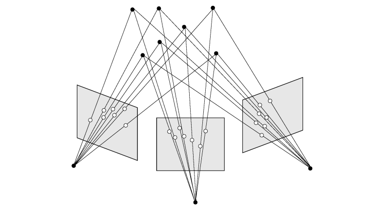
Assume \(n\) 3D points are seen in \(m\) views with \(n = 4, m = 3\).

Let \(\mathbf{x}_{ij}\) be the projection of the \(i\)-th point on image \(j\), \(\mathbf{a}_j\) the vector of parameters for camera \(j\) and \(\mathbf{b}_i\) the vector of parameters for point \(i\).

• BA code (CG)

BA as a NonLinear Least Squares Problem

BA minimizes the reprojection error over all point and camera parameters (\(v_{ij}\) = 1 if point \(i\) is visible in image \(j\))

\[ \min_{\mathbf{a}_{j}, \mathbf{b}_{i}} \sum_{i=1}^{n} \sum_{j=1}^{m} v_{i j} d\left(\mathbf{Q}\left(\mathbf{a}_{j}, \mathbf{b}_{i}\right), \mathbf{x}_{i j}\right)^{2} \]

The parameter vector (6m + 3n)

\[ \mathbf{P}= \left( \mathbf{a}_{1}^{T}, \mathbf{a}_{2}^{T}, \mathbf{a}_{3}^{T} \mid \mathbf{b}_{1}^{T}, \mathbf{b}_{2}^{T}, \mathbf{b}_{3}^{T}, \mathbf{b}_{4}^{T} \right)^{T} \]

The measurement vector (2 * m * n)

\[ \mathbf{X}=\left(\mathbf{x}_{11}^{T}, \mathbf{x}_{12}^{T}, \mathbf{x}_{13}^{T}, \mathbf{x}_{21}^{T}, \mathbf{x}_{22}^{T}, \mathbf{x}_{23}^{T}, \mathbf{x}_{31}^{T}, \mathbf{x}_{32}^{T}, \mathbf{x}_{33}^{T}, \mathbf{x}_{41}^{T}, \mathbf{x}_{42}^{T}, \mathbf{x}_{43}^{T}\right)^{T} \]

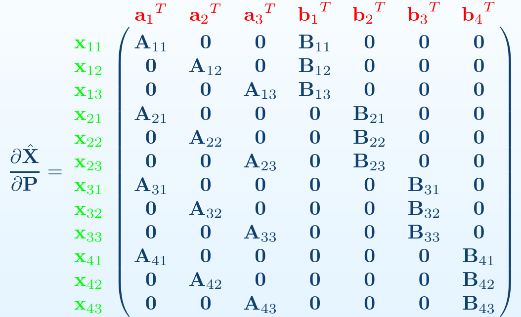
The estimated measurement vector (and do a first-order Taylor expansion)

\[ \begin{aligned} \hat{\mathbf{X}} &= f(\mathbf{P} \oplus \Delta) = \left( \hat{\mathbf{x}}_{11}^{T}, \ldots, \hat{\mathbf{x}}_{1 m}^{T}, \hat{\mathbf{x}}_{21}^{T}, \ldots, \hat{\mathbf{x}}_{2 m}^{T}, \ldots, \hat{\mathbf{x}}_{n 1}^{T}, \ldots, \hat{\mathbf{x}}_{n m}^{T} \right)^{T} \\&= f(a \oplus \delta{a}, b \oplus \delta{b}) \approx f(\mathbf{P}) + \mathbf{A} \delta{a} + \mathbf{B} \delta{b} \end{aligned} \]

with

\[ \hat{\mathbf{x}}_{i j} = \mathbf{Q}\left(\mathbf{a}_{j}, \mathbf{b}_{i} \right) \]

BA corresponds to minimizing the squared \(\Sigma_{\mathbf{X}}^{-1}\)-norm, which is a nonlinear least squares problem

\[ \epsilon^{T} \epsilon = \sum_{i=1}^{4} \sum_{j=1}^{3} \|\epsilon_{ij} \|^{2} = \|\mathbf{X}-\hat{\mathbf{X}}\|^{2} \]

or

\[ \epsilon^{T} \Sigma_{X}^{-1} \epsilon = \| \mathbf{X} - \hat{\mathbf{X}} \|^2_{\Sigma_X} \]

Solved with LM

the augmented normal equation of the LM nonlinear least-squares algorithm

\[ \color{blue} { \left(\mathbf{J}^{T} \Sigma_{X}^{-1} \mathbf{J} + \mu \mathbf{I}\right) \delta= \mathbf{J}^{T} \Sigma_{X}^{-1} \epsilon } \]

The LM updating vector

\[ \delta \triangleq \left(\delta_{\mathbf{a}}^{T}, \delta_{\mathbf{b}}^{T}\right)^{T} \triangleq \left(\delta_{\mathbf{a}_{1}}^{T}, \delta_{\mathbf{a}_{2}}^{T}, \delta_{\mathbf{a}_{3}}^{T}, \delta_{\mathbf{b}_{1}}^{T}, \delta_{\mathbf{b}_{2}}^{T}, \delta_{\mathbf{b}_{3}}^{T}, \delta_{\mathbf{b}_{4}}^{T}\right)^{T} \]

The Jacobian Matrix \(\mathbf{J}\) in block form

\[ \mathbf{J} = \frac{\partial \hat{\mathbf{X}}}{\partial \mathbf{P}} = \left[ \frac{\partial \hat{\mathbf{X}}}{\partial \mathbf{a}} \mid \frac{\partial \hat{\mathbf{X}}}{\partial \mathbf{b}} \right] = \left[ \mathbf{A} \mid \mathbf{B} \right] \]

with

\[ \mathbf{A}_{i j} \triangleq \frac{\partial \hat{\mathbf{x}}_{i j}}{\partial \mathbf{a}_{k}} = \mathbf{0}, \forall j \neq k \]

\[ \mathbf{B}_{i j} \triangleq \frac{\partial \hat{\mathbf{x}}_{i j}}{\partial \mathbf{b}_{k}} = \mathbf{0}, \forall i \neq k \]

the Covariance Matrix \(\Sigma\)

\[ \Sigma_{\mathbf{X}} = \operatorname{diag}\left(\Sigma_{\mathbf{x}_{11}}, \Sigma_{\mathbf{x}_{12}}, \Sigma_{\mathbf{x}_{13}}, \Sigma_{\mathbf{x}_{21}}, \Sigma_{\mathbf{x}_{22}}, \Sigma_{\mathbf{x}_{23}}, \Sigma_{\mathbf{x}_{31}}, \Sigma_{\mathbf{x}_{32}}, \Sigma_{\mathbf{x}_{33}}, \Sigma_{\mathbf{x}_{41}}, \Sigma_{\mathbf{x}_{42}}, \Sigma_{\mathbf{x}_{43}}\right) \]

the Hessian or Information Matrix \(\mathbf{H}\), the left-hand side of above augmented normal equation

\[ \mathbf{J}^{T} \Sigma_{\mathbf{X}}^{-1} \mathbf{J} = \left(\begin{array}{ccccccc} \mathbf{U}_{1} & \mathbf{0} & \mathbf{0} & \mathbf{W}_{11} & \mathbf{W}_{21} & \mathbf{W}_{31} & \mathbf{W}_{41} \\ \mathbf{0} & \mathbf{U}_{2} & \mathbf{0} & \mathbf{W}_{12} & \mathbf{W}_{22} & \mathbf{W}_{32} & \mathbf{W}_{42} \\ \mathbf{0} & \mathbf{0} & \mathbf{U}_{3} & \mathbf{W}_{13} & \mathbf{W}_{23} & \mathbf{W}_{33} & \mathbf{W}_{43} \\ \mathbf{W}_{11}^{T} & \mathbf{W}_{12}^{T} & \mathbf{W}_{13}^{T} & \mathbf{V}_{1} & \mathbf{0} & \mathbf{0} & \mathbf{0} \\ \mathbf{W}_{21}^{T} & \mathbf{W}_{22}^{T} & \mathbf{W}_{23}^{T} & \mathbf{0} & \mathbf{V}_{2} & \mathbf{0} & \mathbf{0} \\ \mathbf{W}_{31}^{T} & \mathbf{W}_{32}^{T} & \mathbf{W}_{33}^{T} & \mathbf{0} & \mathbf{0} & \mathbf{V}_{3} & \mathbf{0} \\ \mathbf{W}_{41}^{T} & \mathbf{W}_{42}^{T} & \mathbf{W}_{43}^{T} & \mathbf{0} & \mathbf{0} & \mathbf{0} & \mathbf{V}_{4} \end{array}\right) \]

with

\[ \begin{aligned} \mathbf{U}_{j} & \equiv \sum_{i=1}^{4} \mathbf{A}_{i j}^{T} \Sigma_{\mathbf{x}_{i j}}^{-1} \mathbf{A}_{i j}, \\ \mathbf{V}_{i} & \equiv \sum_{j=1}^{3} \mathbf{B}_{i j}^{T} \Sigma_{\mathbf{x}_{i j}}^{-1} \mathbf{B}_{i j}, \\ \mathbf{W}_{i j} & \equiv \mathbf{A}_{i j}^{T} \Sigma_{\mathbf{x}_{i j}}^{-1} \mathbf{B}_{i j} \end{aligned} \]

the right-hand side of above augmented normal equation

\[ \mathbf{J}^{T} \Sigma_{\mathbf{X}}^{-1} \epsilon = \begin{bmatrix} \sum_{i=1}^{4}\left(\mathbf{A}_{i 1}^{T} \Sigma_{\mathbf{x}_{i} 1}^{-1} \epsilon_{i 1}\right) \\[5pt] \sum_{i=1}^{4}\left(\mathbf{A}_{i 2}^{T} \Sigma_{\mathbf{x}_{i} 2}^{-1} \epsilon_{i 2}\right) \\[5pt] \sum_{i=1}^{4}\left(\mathbf{A}_{i 3}^{T} \Sigma_{\mathbf{x}_{i} 3}^{-1} \epsilon_{i 3}\right) \\[5pt] \sum_{j=1}^{3}\left(\mathbf{B}_{1 j}^{T} \Sigma_{\mathbf{x}_{1 j}}^{-1} \epsilon_{1 j}\right) \\[5pt] \sum_{j=1}^{3}\left(\mathbf{B}_{2 j}^{T} \Sigma_{\mathbf{x}_{2 j}}^{-1} \epsilon_{2 j}\right) \\[5pt] \sum_{j=1}^{3}\left(\mathbf{B}_{3 j}^{T} \Sigma_{\mathbf{x}_{3 j}}^{-1} \epsilon_{3 j}\right) \\[5pt] \sum_{j=1}^{3}\left(\mathbf{B}_{4 j}^{T} \Sigma_{\mathbf{x}_{4 j}}^{-1} \epsilon_{4 j}\right) \end{bmatrix} \]

we can get with all above equations

\[ \left(\begin{array}{ccc|cccc} \mathbf{U}_{1} & \mathbf{0} & \mathbf{0} & \mathbf{W}_{11} & \mathbf{W}_{21} & \mathbf{W}_{31} & \mathbf{W}_{41} \\ \mathbf{0} & \mathbf{U}_{2} & \mathbf{0} & \mathbf{W}_{12} & \mathbf{W}_{22} & \mathbf{W}_{32} & \mathbf{W}_{42} \\ \mathbf{0} & \mathbf{0} & \mathbf{U}_{3} & \mathbf{W}_{13} & \mathbf{W}_{23} & \mathbf{W}_{33} & \mathbf{W}_{43} \\ \hline \mathbf{W}_{11}^{T} & \mathbf{W}_{12}^{T} & \mathbf{W}_{13}^{T} & \mathbf{V}_{1} & \mathbf{0} & \mathbf{0} & \mathbf{0} \\ \mathbf{W}_{21}^{T} & \mathbf{W}_{22}^{T} & \mathbf{W}_{23}^{T} & \mathbf{0} & \mathbf{V}_{2} & \mathbf{0} & \mathbf{0} \\ \mathbf{W}_{31}^{T} & \mathbf{W}_{32}^{T} & \mathbf{W}_{33}^{T} & \mathbf{0} & \mathbf{0} & \mathbf{V}_{3} & \mathbf{0} \\ \mathbf{W}_{41}^{T} & \mathbf{W}_{42}^{T} & \mathbf{W}_{43}^{T} & \mathbf{0} & \mathbf{0} & \mathbf{0} & \mathbf{V}_{4} \end{array}\right) \left(\begin{array}{c} \delta_{\mathbf{a}_{1}} \\ \delta_{\mathbf{a}_{2}} \\ \delta_{\mathbf{a}_{3}} \\ \delta_{\mathbf{b}_{1}} \\ \delta_{\mathbf{b}_{2}} \\ \delta_{\mathbf{b}_{3}} \\ \delta_{\mathbf{b}_{4}} \end{array}\right)= \left(\begin{array}{c} \epsilon_{\mathbf{a}_{1}} \\ \epsilon_{\mathbf{a}_{2}} \\ \epsilon_{\mathbf{a}_{3}} \\ \epsilon_{\mathbf{b}_{1}} \\ \epsilon_{\mathbf{b}_{2}} \\ \epsilon_{\mathbf{b}_{3}} \\ \epsilon_{\mathbf{b}_{4}} \end{array}\right) \]

or

\[ \left[\begin{array}{c|c} \mathbf{A}^{T} \mathbf{A} & \mathbf{A}^{T} \mathbf{B} \\ \hline \mathbf{B}^{T} \mathbf{A} & \mathbf{B}^{T} \mathbf{B} \end{array}\right]\left(\frac{\delta_{\mathbf{a}}}{\delta_{\mathbf{b}}}\right)=\left(\frac{\mathbf{A}^{T} \epsilon}{\mathbf{B}^{T} \epsilon}\right) \]

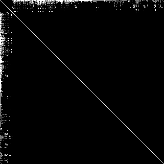
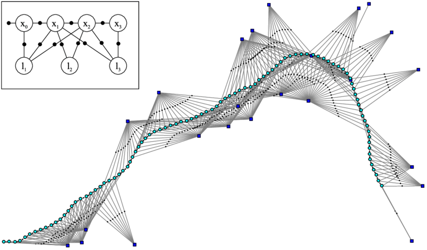
\(\mathbf{J}^T \mathbf{J}\) sparsity pattern

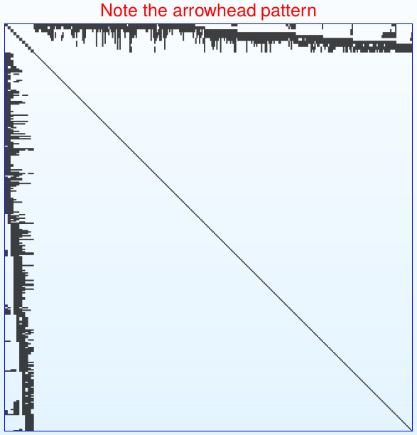
Draw Hessian matrix sparsity pattern from BAL Problem (code):

const int num_points        = bal_problem->num_points();
const int num_cameras       = bal_problem->num_cameras();
const int num_observations  = bal_problem->num_observations();

std::vector<int> idx_obs;
idx_obs.reserve(num_observations);
for (int i = 0; i < num_observations; ++i) {
    const int camera_id = bal_problem->camera_index()[i];
    const int point_id = bal_problem->point_index()[i];

    if (point_id >= max_point_id)
        continue;

    idx_obs.push_back(i);
}

const int j_rows = idx_obs.size();
const int j_cols = num_cameras + max_point_id;

Eigen::MatrixXi mJ(j_rows, j_cols);
mJ.setZero();

for (int i = 0; i < idx_obs.size(); ++i) {
    int j = idx_obs[i];
    const int camera_id = bal_problem->camera_index()[j];
    const int point_id = bal_problem->point_index()[j];
    // std::cout << camera_id << ", " << point_id << std::endl;
    mJ(i, camera_id) = 1;
    mJ(i, num_cameras + point_id) = 1;
}

Eigen::MatrixXi mH = mJ.transpose() * mJ;

cv::Mat mat_H(mH.rows(), mH.cols(), CV_8UC1);
for (int y = 0; y < mH.rows(); ++y) {
    for (int x = 0; x < mH.cols(); ++x) {
        mat_H.at<unsigned char>(y, x) = mH(y, x);
    }
}
cv::threshold(mat_H, mat_H, 0, 255, cv::THRESH_BINARY);

Solving the augmented normal equations

The augmented normal equations take the form

\[ \left(\begin{array}{cc} \mathbf{U}^{*} & \mathbf{W} \\ \mathbf{W}^{T} & \mathbf{V}^{*} \end{array}\right)\left(\begin{array}{l} \delta_{\mathbf{a}} \\ \delta_{\mathbf{b}} \end{array}\right)=\left(\begin{array}{c} \epsilon_{\mathbf{a}} \\ \epsilon_{\mathbf{b}} \end{array}\right) \]

Solve \(\delta \mathbf{a}\) (Marginalize 3D Points)

Performing block Gaussian elimination in the lhs matrix, \(\delta \mathbf{a}\) is determined with Cholesky from \(\mathbf{V}^{*}\)’s Schur complement:

\[ \left(\mathbf{U}^{*}-\mathbf{W} \mathbf{V}^{*-1} \mathbf{W}^{T}\right) \delta_{\mathbf{a}}=\epsilon_{\mathbf{a}}-\mathbf{W} \mathbf{V}^{*-1} \epsilon_{\mathbf{b}} \]

with

\[ \mathbf{V}^{*-1}= \left(\begin{array}{ccc} \mathbf{V}_{1}^{*-1} & \mathbf{0} & \cdots \\ \mathbf{0} & \mathbf{V}_{2}^{*-1} & \cdots \\ \vdots & \vdots & \ddots \end{array}\right) \]

Why solve for \(\delta \mathbf{a}\) first? Typically \(m<<n\).

Solve \(\delta \mathbf{b}\)

\(\delta \mathbf{b}\) can be computed by back substitution into

\[ \mathbf{V}^{*} \delta_{\mathbf{b}} = \epsilon_{\mathbf{b}}-\mathbf{W}^{T} \delta_{\mathbf{a}} \]

the Reduced Camera Matrix

\[ \mathbf{S} \equiv \mathbf{U}^{*}-\mathbf{W} \mathbf{V}^{*-1} \mathbf{W}^{T} \]

• The lhs matrix \(\mathbf{S}\) is referred to as the reduced camera matrix (RCM)

• Since not all scene points appear in all cameras, \(\mathbf{S}\) is sparse. This is known as secondary structure.

• Dealing with the RCM
  • Store as dense, decompose with ordinary linear algebra
    • SBA: A software package for generic sparse bundle adjustment
    • cvsba: an OpenCV wrapper for sba library
  • Store as sparse, factorize with sparse direct solvers
    • Sparse Sparse Bundle Adjustment
  • Store as sparse, use conjugate gradient methods
    • Bundle Adjustment in the Large
  • Avoid storing altogether
    • Multicore Bundle Adjustment

Reducing the cost of BA

• reducing BA’s size
  • BA in a sliding time window (local BA)
• reducing frequency of invocation
  • Solve the RCM fewer times: Dog-leg in place of LM

手撸 BA

Optimization Libraries

• Ceres-Solver
• G2O
• GTSAM

Others

Factor Graph

因子图 是用来分析SFM/SLAM问题结构的一种常用的 概率图 工具。因子图是 二分图，包含节点和边，一般 节点 表示优化变量，边 表示约束。

Motion only BA (Pose Graph Optimization)

在BA中，三维点的变量数一般会远大于相机的变量数，导致求解的线性方程组的规模非常大，即使利用稀疏性求解复杂度依然很高。因此 位姿图优化算法（Lu et al., 1997a）被提出来以提高全局优化的效率。

• Pose Graph Optimization
• Robust Factor Graphs for Pose Graph SLAM

Incremental BA

基于贝叶斯推断的增量式BA

• iSAM (Incremental Smoothing and Mapping) is an optimization library for sparse nonlinear problems as encountered in simultaneous localization and mapping (SLAM), provides efficient algorithms for batch and incremental optimization, recovering the exact least-squares solution

• iSAM2

基于增量更新舒尔补的增量式BA

• zju3dv/EIBA: Efficient Incremental BA, which is part of our RKD-SLAM

• baidu/ICE-BA: Incremental, Consistent and Efficient Bundle Adjustment for Visual-Inertial SLAM

• SLAM++

References

• SBA: A software package for generic sparse bundle adjustment
• Bundle adjustment gone public (slides)
• 增强现实：原理、算法与应用