Multi-Sensor Fusion: IMU and GPS loose fusion based on ESKF

[TOC]

Overview

• 代码：imu_x_fusion

System State Vector

the nominal-state \(\mathbf{x}\) and the error-state \(\delta \mathbf{x}\)

\[ \mathbf{x} = \begin{bmatrix} \mathbf{p} \\ \mathbf{v} \\ \mathbf{q} \\ \mathbf{b}_a \\ \mathbf{b}_g \end{bmatrix} \in \mathbb{R}^{16 \times 1} \quad \delta \mathbf{x} = \begin{bmatrix} \delta \mathbf{p} \\ \delta \mathbf{v} \\ \delta \boldsymbol{\theta} \\ \delta \mathbf{b}_a \\ \delta \mathbf{b}_g \end{bmatrix} \in \mathbb{R}^{15 \times 1} \]

the true-state

\[ \mathbf{x}_{t} = \mathbf{x} \oplus \delta \mathbf{x} \]

ENU Coordinate

• using ENU coordinate
• in ENU coordinate, \(\mathbf{g} = \begin{bmatrix} 0 & 0 & -9.81007 \end{bmatrix}^T\)
• extrinsic between IMU and GPS: \({}^{I} \mathbf{p}_{G p s}\)

State Prediction (IMU-driven system kinematics in discrete time)

The nominal state kinematics

\[ \begin{array}{l} \mathbf{p} \leftarrow \mathbf{p}+\mathbf{v} \Delta t+\frac{1}{2}\left(\mathbf{R}\left(\mathbf{a}_{m}-\mathbf{a}_{b}\right)+\mathbf{g}\right) \Delta t^{2} \\ \mathbf{v} \leftarrow \mathbf{v}+\left(\mathbf{R}\left(\mathbf{a}_{m}-\mathbf{a}_{b}\right)+\mathbf{g}\right) \Delta t \\ \mathbf{q} \leftarrow \mathbf{q} \otimes \mathbf{q}\left\{\left(\boldsymbol{\omega}_{m}-\boldsymbol{\omega}_{b}\right) \Delta t\right\} \\ \mathbf{a}_{b} \leftarrow \mathbf{a}_{b} \\ \boldsymbol{\omega}_{b} \leftarrow \boldsymbol{\omega}_{b} \end{array} \]

The error-state kinematics

\[ \begin{aligned} \delta \mathbf{p} & \leftarrow \delta \mathbf{p}+\delta \mathbf{v} \Delta t \\ \delta \mathbf{v} & \leftarrow \delta \mathbf{v}+\left(-\mathbf{R}\left[\mathbf{a}_{m}-\mathbf{a}_{b}\right]_{\times} \delta \boldsymbol{\theta}-\mathbf{R} \delta \mathbf{a}_{b}+\delta \mathbf{g}\right) \Delta t+\mathbf{v}_{\mathbf{i}} \\ \delta \boldsymbol{\theta} & \leftarrow \mathbf{R}^{\top}\left\{\left(\boldsymbol{\omega}_{m}-\boldsymbol{\omega}_{b}\right) \Delta t\right\} \delta \boldsymbol{\theta}-\delta \boldsymbol{\omega}_{b} \Delta t+\boldsymbol{\theta}_{\mathbf{i}} \\ \delta \mathbf{a}_{b} & \leftarrow \delta \mathbf{a}_{b}+\mathbf{a}_{\mathbf{i}} \\ \delta \boldsymbol{\omega}_{b} & \leftarrow \delta \boldsymbol{\omega}_{b}+\boldsymbol{\omega}_{\mathbf{i}} \\ \delta \mathbf{g} & \leftarrow \delta \mathbf{g} \end{aligned} \]

The error-state Jacobian and perturbation matrices

The error-state system is now

\[ \delta \mathbf{x} \leftarrow f\left(\mathbf{x}, \delta \mathbf{x}, \mathbf{u}_{m}, \mathbf{i}\right)=\mathbf{F}_{\mathbf{x}}\left(\mathbf{x}, \mathbf{u}_{m}\right) \cdot \delta \mathbf{x}+\mathbf{F}_{\mathbf{i}} \cdot \mathbf{i} \]

The ESKF prediction equations are written:

\[ \begin{array}{l} \hat{\delta \mathbf{x}} \leftarrow \mathbf{F}_{\mathbf{x}}\left(\mathbf{x}, \mathbf{u}_{m}\right) \cdot \hat{\delta \mathbf{x}} \\ \mathbf{P} \leftarrow \mathbf{F}_{\mathbf{x}} \mathbf{P} \mathbf{F}_{\mathbf{x}}^{\top}+\mathbf{F}_{\mathbf{i}} \mathbf{Q}_{\mathbf{i}} \mathbf{F}_{\mathbf{i}}^{\top} \end{array} \]

\[ \delta \mathbf{x} \sim \mathcal{N}\{\hat{\delta} \mathbf{x}, \mathbf{P}\} \]

where

\[ \mathbf{F}_{\mathbf{x}} = \left.\frac{\partial f}{\partial \delta \mathbf{x}}\right|_{\mathbf{x}, \mathbf{u}_{m}} = \left[\begin{array}{ccccc} \mathbf{I} & \mathbf{I} \Delta t & 0 & 0 & 0 \\ 0 & \mathbf{I} & -\mathbf{R}\left[\mathbf{a}_{m}-\mathbf{a}_{b}\right]_{\times} \Delta t & -\mathbf{R} \Delta t & 0 \\ 0 & 0 & \mathbf{R}^{\top}\left\{\left(\boldsymbol{\omega}_{m}-\boldsymbol{\omega}_{b}\right) \Delta t\right\} & 0 & - \mathbf{I} \Delta t \\ 0 & 0 & 0 & \mathbf{I} & 0 \\ 0 & 0 & 0 & 0 & \mathbf{I} \end{array}\right] \]

\[ \mathbf{F}_{\mathbf{i}}= \left.\frac{\partial f}{\partial \mathbf{i}}\right|_{\mathbf{x}, \mathbf{u}_{m}}= \left[\begin{array}{llll} 0 & 0 & 0 & 0 \\ \mathbf{I} & 0 & 0 & 0 \\ 0 & \mathbf{I} & 0 & 0 \\ 0 & 0 & \mathbf{I} & 0 \\ 0 & 0 & 0 & \mathbf{I} \end{array}\right] \]

\[ \mathbf{Q}_{\mathbf{i}}= \left[\begin{array}{cccc} \mathbf{V}_{\mathbf{i}} & 0 & 0 & 0 \\ 0 & \boldsymbol{\Theta}_{\mathbf{i}} & 0 & 0 \\ 0 & 0 & \mathbf{A}_{\mathbf{i}} & 0 \\ 0 & 0 & 0 & \Omega_{\mathbf{i}} \end{array}\right] \]

where

\[ \begin{array}{ll} \mathbf{V}_{\mathbf{i}}=\sigma_{\tilde{\mathbf{a}}_{n}}^{2} \Delta t^{2} \mathbf{I} & {\left[m^{2} / s^{2}\right]} \\ \Theta_{\mathbf{i}}=\sigma_{\tilde{\boldsymbol{\omega}}_{n}}^{2} \Delta t^{2} \mathbf{I} & {\left[r a d^{2}\right]} \\ \mathbf{A}_{\mathbf{i}}=\sigma_{\mathbf{a}_{w}}^{2} \Delta t \mathbf{I} & {\left[m^{2} / s^{4}\right]} \\ \boldsymbol{\Omega}_{\mathbf{i}}=\sigma_{\boldsymbol{\omega}_{w}}^{2} \Delta t \mathbf{I} & {\left[r a d^{2} / s^{2}\right]} \end{array} \]

ESKF Measurement Update (Fusing IMU with GPS data)

GPS measurement

\[ \mathbf{y}=h\left(\mathbf{x}_{t}\right)+v , \quad v \sim \mathcal{N}\{0, \mathbf{V}\} \]

convert the GPS raw data which is in WGS84 coordinate to ENU by GeographicLib

\[ h\left(\hat{\mathbf{x}}_{t}\right) = {}^{G} \mathbf{p}_{G p s} = {}^{G} \mathbf{p}_{I} + {}_{I}^{G} \mathbf{R} \cdot {}^{I} \mathbf{p}_{G p s} \]

the filter correction equations

\[ \begin{array}{l} \mathbf{K}=\mathbf{P} \mathbf{H}^{\top}\left(\mathbf{H} \mathbf{P} \mathbf{H}^{\top}+\mathbf{V}\right)^{-1} \\ \hat{\delta} \mathbf{x} \leftarrow \mathbf{K}\left(\mathbf{y}-h\left(\hat{\mathbf{x}}_{t}\right)\right) \\ \mathbf{P} \leftarrow(\mathbf{I}-\mathbf{K} \mathbf{H}) \mathbf{P} \end{array} \]

where

\[ \mathbf{H} \left.\triangleq \frac{\partial h}{\partial \delta \mathbf{x}}\right|_{\mathbf{x}} = \left[\begin{array}{lll} \mathbf{I} & \mathbf{0} & -{}_{I}^{G} \mathbf{R} \lfloor {}^{I} \mathbf{p}_{G p s} \rfloor _{\times} & \mathbf{0} & \mathbf{0} \end{array}\right] \]

the best true-state estimate

\[ \hat{\mathbf{x}}_{t}=\mathbf{x} \oplus \hat{\delta} \mathbf{x} \]

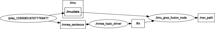
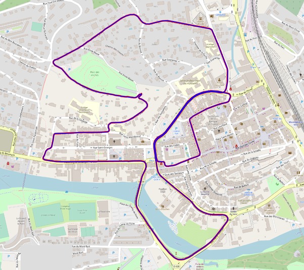
Results

path on ROS rviz and plot the result path(fusion_gps.csv & fusion_state.csv) on google map:

Reference

• Quaternion kinematics for the error-state Kalman filter