计算机视觉对极几何之Triangulate

[TOC]

极线搜索

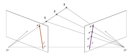
If we are using only the left camera, we can't find the 3D point corresponding to the point \(x\) in image because every point on the line \(OX\) projects to the same point on the image plane. But consider the right image also. Now different points on the line \(OX\) projects to different points ( \(x^{\prime}\)) in right plane. So with these two images, we can triangulate the correct 3D point.

The projection of the different points on \(OX\) form a line on right plane (line \(l^{\prime}\)). We call it epiline corresponding to the point \(x\). It means, to find the point \(x\) on the right image, search along this epiline. It should be somewhere on this line (Think of it this way, to find the matching point in other image, you need not search the whole image, just search along the epiline. So it provides better performance and accuracy). This is called Epipolar Constraint. Similarly all points will have its corresponding epilines in the other image.

• epiline: \(l\), \(l^{\prime}\)
• epipole: \(e\), \(e^{\prime}\)
• epipolar plane: \(XOO^{\prime}\)

求解空间点坐标

ORB-SLAM2

已知，两个视图下匹配点的 图像坐标 \(\boldsymbol{p}_1\) 和 \(\boldsymbol{p}_2\)，两个相机的相对位姿 \(\boldsymbol{T}\) ，相机内参矩阵 \(\boldsymbol{K}\)，求 对应的三维点坐标 \(\boldsymbol{P}\)，其齐次坐标为 \(\tilde{\boldsymbol{P}}\)。

相对位姿

\[ \boldsymbol{T} = \boldsymbol{T}_{21} = [ \boldsymbol{R} \quad \boldsymbol{t} ] \in \mathbb{R}^{3 \times 4} \]

两个视图的 投影矩阵 分别为

\[ \boldsymbol{P}_1 = \boldsymbol{K} \cdot [\boldsymbol{I}_{3 \times 3} \quad \mathbf{0}_{3 \times 1}], \quad \boldsymbol{P}_1 \in \mathbb{R}^{3 \times 4} \]

\[ \boldsymbol{P}_2 = \boldsymbol{K} \cdot [ \boldsymbol{R}_{3 \times 3} \quad \boldsymbol{t}_{3 \times 1} ], \quad \boldsymbol{P}_2 \in \mathbb{R}^{3 \times 4} \]

由于是齐次坐标的表示形式，使用叉乘消去齐次因子

\[ \tilde{\boldsymbol{p}_1} \times (\boldsymbol{P}_1 \tilde{\boldsymbol{P}}) = \mathbf{0} \]

\[ \tilde{\boldsymbol{p}_2} \times (\boldsymbol{P}_2 \tilde{\boldsymbol{P}}) = \mathbf{0} \]

把 \(\boldsymbol{P}_1\) 和 \(\boldsymbol{P}_2\) 按行展开（上标代表行索引）代入，对于第一视图有

\[ \begin{bmatrix} 0 & -1 & v_1 \\ 1 & 0 & -u_1 \\ -v_1 & u_1 & 0 \end{bmatrix} \cdot \begin{bmatrix} \boldsymbol{P}_1^1 \cdot \tilde{\boldsymbol{P}} \\ \boldsymbol{P}_1^2 \cdot \tilde{\boldsymbol{P}} \\ \boldsymbol{P}_1^3 \cdot \tilde{\boldsymbol{P}} \end{bmatrix} = \mathbf{0} \]

即

\[ \begin{aligned} u_1 (\boldsymbol{P}_1^3 \cdot \tilde{\boldsymbol{P}}) - (\boldsymbol{P}_1^1 \cdot \tilde{\boldsymbol{P}}) = 0 \\ v_1 (\boldsymbol{P}_1^3 \cdot \tilde{\boldsymbol{P}}) - (\boldsymbol{P}_1^2 \cdot \tilde{\boldsymbol{P}}) = 0 \\ u_1 (\boldsymbol{P}_1^2 \cdot \tilde{\boldsymbol{P}}) - v_1 (\boldsymbol{P}_1^1 \cdot \tilde{\boldsymbol{P}}) = 0 \\ \end{aligned} \]

可见第三个式子可以由上两个式子线性表示，所以只需要取前连个式子即可

\[ \begin{bmatrix} u_1 \boldsymbol{P}_1^3 - \boldsymbol{P}_1^1 \\ v_1 \boldsymbol{P}_1^3 - \boldsymbol{P}_1^2 \end{bmatrix} \cdot \tilde{\boldsymbol{P}} = \mathbf{0} \]

同样的，对于第二视图

\[ \begin{bmatrix} u_2 \boldsymbol{P}_2^3 - \boldsymbol{P}_2^1 \\ v_2 \boldsymbol{P}_2^3 - \boldsymbol{P}_2^2 \end{bmatrix} \cdot \tilde{\boldsymbol{P}} = \mathbf{0} \]

组合起来

\[ \boldsymbol{A_{4 \times 4}} \cdot \tilde{\boldsymbol{P}} = \begin{bmatrix} u_1 \boldsymbol{P}_1^3 - \boldsymbol{P}_1^1 \\ v_1 \boldsymbol{P}_1^3 - \boldsymbol{P}_1^2 \\ u_2 \boldsymbol{P}_2^3 - \boldsymbol{P}_2^1 \\ v_2 \boldsymbol{P}_2^3 - \boldsymbol{P}_2^2 \end{bmatrix} \cdot \tilde{\boldsymbol{P}} = \mathbf{0} \]

求解 \(\boldsymbol{P}\) 相当于解一个 线性最小二乘问题。

SVD分解 \(\boldsymbol{A}\)

\[ \text{SVD}(\boldsymbol{A}) = \boldsymbol{U} \boldsymbol{\Sigma} \boldsymbol{V}^T \]

方程的解为 \(\boldsymbol{A}\) 的 最小奇异值 对应的 奇异矢量，即 齐次坐标

\[ \tilde{\boldsymbol{P}} = (X,Y,Z,W) = \boldsymbol{V}_3 \]

最终，\(\boldsymbol{P}\)（第一视图坐标系下三维坐标）为

\[ \boldsymbol{P} = (\frac{X}{W}, \frac{Y}{W}, \frac{Z}{W}) \]

示例代码1

void Initializer::Triangulate(
  const cv::KeyPoint &kp1,
  const cv::KeyPoint &kp2,
  const cv::Mat &P1,
  const cv::Mat &P2,
  cv::Mat &x3D)
{
    cv::Mat A(4,4,CV_32F);

    A.row(0) = kp1.pt.x*P1.row(2)-P1.row(0);
    A.row(1) = kp1.pt.y*P1.row(2)-P1.row(1);
    A.row(2) = kp2.pt.x*P2.row(2)-P2.row(0);
    A.row(3) = kp2.pt.y*P2.row(2)-P2.row(1);

    cv::Mat u,w,vt;
    cv::SVD::compute(A,w,u,vt,cv::SVD::MODIFY_A| cv::SVD::FULL_UV);
    x3D = vt.row(3).t();
    x3D = x3D.rowRange(0,3)/x3D.at<float>(3);
}

示例代码2

const cv::KeyPoint &kp1 = mpCurrentKeyFrame->mvKeysUn[idx1];
const cv::KeyPoint &kp2 = pKF2->mvKeysUn[idx2];

cv::Mat xn1 = (cv::Mat_<float>(3,1) << (kp1.pt.x-cx1)*invfx1, (kp1.pt.y-cy1)*invfy1, 1.0);
cv::Mat xn2 = (cv::Mat_<float>(3,1) << (kp2.pt.x-cx2)*invfx2, (kp2.pt.y-cy2)*invfy2, 1.0);

// Linear Triangulation Method
cv::Mat A(4,4,CV_32F);
A.row(0) = xn1.at<float>(0)*Tcw1.row(2)-Tcw1.row(0);
A.row(1) = xn1.at<float>(1)*Tcw1.row(2)-Tcw1.row(1);
A.row(2) = xn2.at<float>(0)*Tcw2.row(2)-Tcw2.row(0);
A.row(3) = xn2.at<float>(1)*Tcw2.row(2)-Tcw2.row(1);

cv::Mat w,u,vt;
cv::SVD::compute(A,w,u,vt,cv::SVD::MODIFY_A| cv::SVD::FULL_UV);

x3D = vt.row(3).t();

if(x3D.at<float>(3)==0)
    continue;

// Euclidean coordinates
x3D = x3D.rowRange(0,3)/x3D.at<float>(3);

Note:

• 示例2代码与PTAM原理一致，相关理论分析见下方PTAM部分

PTAM

已知，两个视图下匹配点的 归一化平面(z=1) (去畸变后) 齐次坐标 \(\boldsymbol{p}_1\) 和 \(\boldsymbol{p}_2\)，两个相机的相对位姿 \(\boldsymbol{T}\)，求 对应的三维点坐标 \(\boldsymbol{P}\)（第一视图坐标系下三维坐标），其齐次坐标为 \(\tilde{\boldsymbol{P}}\)。

方程

\[ \boldsymbol{p}_1 \times (\boldsymbol{I}_{3 \times 4} \cdot \tilde{\boldsymbol{P}}) = \mathbf{0} \]

\[ \boldsymbol{p}_2 \times (\boldsymbol{T}_{21} \cdot \tilde{\boldsymbol{P}}) = \mathbf{0} \]

\[ \boldsymbol{T} = \boldsymbol{T}_{21} = [ \boldsymbol{R} \quad \boldsymbol{t} ] \in \mathbb{R}^{3 \times 4} \]

矩阵形式

\[ \boldsymbol{A_{6 \times 4}} \cdot \tilde{\boldsymbol{P}} = \begin{bmatrix} \boldsymbol{p}_1 \times \boldsymbol{I}_{3 \times 4} \\ \boldsymbol{p}_2 \times \boldsymbol{T}_{21} \end{bmatrix} \cdot \tilde{\boldsymbol{P}} = \mathbf{0} \]

求解 \(\boldsymbol{P}\) 相当于解一个 线性最小二乘问题。

SVD分解 \(\boldsymbol{A}\)

\[ \text{SVD}(\boldsymbol{A}) = \boldsymbol{U} \boldsymbol{\Sigma} \boldsymbol{V}^T \]

方程的解为 \(\boldsymbol{A}\) 的 最小奇异值 对应的 奇异矢量，即 齐次坐标

\[ \tilde{\boldsymbol{P}} = (X,Y,Z,W) = \boldsymbol{V}_3 \]

最终，\(\boldsymbol{P}\)（第一视图坐标系下三维坐标）为

\[ \boldsymbol{P} = (\frac{X}{W}, \frac{Y}{W}, \frac{Z}{W}) \]

ptam_cg中示例代码Triangulate：

Vector<3> MapMaker::Triangulate(
  SE3<> se3AfromB,
  const Vector<2> &v2A,
  const Vector<2> &v2B)
{
    Matrix<3,4> PDash;
    PDash.slice<0,0,3,3>() = se3AfromB.get_rotation().get_matrix();
    PDash.slice<0,3,3,1>() = se3AfromB.get_translation().as_col();

    Matrix<4> A;
    A[0][0] = -1.0; A[0][1] =  0.0; A[0][2] = v2B[0]; A[0][3] = 0.0;
    A[1][0] =  0.0; A[1][1] = -1.0; A[1][2] = v2B[1]; A[1][3] = 0.0;
    A[2] = v2A[0] * PDash[2] - PDash[0];
    A[3] = v2A[1] * PDash[2] - PDash[1];

    SVD<4,4> svd(A);
    Vector<4> v4Smallest = svd.get_VT()[3];
    if(v4Smallest[3] == 0.0)
        v4Smallest[3] = 0.00001;
    return project(v4Smallest);
}

ptam_cg中示例代码TriangulateNew：

Vector<3> MapMaker::TriangulateNew(
  SE3<> se3AfromB,
  const Vector<2> &v2A,
  const Vector<2> &v2B)
{
    Vector<3> v3A = unproject(v2A);
    Vector<3> v3B = unproject(v2B);

    Matrix<3> m3A = TooN::Zeros;
    m3A[0][1] = -v3A[2];
    m3A[0][2] =  v3A[1];
    m3A[1][2] = -v3A[0];
    m3A[1][0] = -m3A[0][1];
    m3A[2][0] = -m3A[0][2];
    m3A[2][1] = -m3A[1][2];
    Matrix<3> m3B = TooN::Zeros;
    m3B[0][1] = -v3B[2];
    m3B[0][2] =  v3B[1];
    m3B[1][2] = -v3B[0];
    m3B[1][0] = -m3B[0][1];
    m3B[2][0] = -m3B[0][2];
    m3B[2][1] = -m3B[1][2];

    Matrix<3,4> m34AB;
    m34AB.slice<0,0,3,3>() = se3AfromB.get_rotation().get_matrix();
    m34AB.slice<0,3,3,1>() = se3AfromB.get_translation().as_col();

    SE3<> se3I;
    Matrix<3,4> m34I;
    m34I.slice<0,0,3,3>() = se3I.get_rotation().get_matrix();
    m34I.slice<0,3,3,1>() = se3I.get_translation().as_col();

    Matrix<3,4> PDashA = m3A * m34AB;
    Matrix<3,4> PDashB = m3B * m34I;

    Matrix<6,4> A;
    A.slice<0,0,3,4>() = PDashA;
    A.slice<3,0,3,4>() = PDashB;

    SVD<6,4> svd(A);
    Vector<4> v4Smallest = svd.get_VT()[3];
    if(v4Smallest[3] == 0.0)
        v4Smallest[3] = 0.00001;

    return project(v4Smallest);
}

求解空间点深度 ^[1]

已知，两个视图下匹配点的 归一化平面(z=1) (去畸变后) 齐次坐标 \(\boldsymbol{p}_1\) 和 \(\boldsymbol{p}_2\)，两个相机的相对位姿 \(\boldsymbol{T}\)，求解空间点深度 \(Z_1\) 和 \(Z_2\)

\[ \boldsymbol{T} = \boldsymbol{T}_{21} = [ \boldsymbol{R} \quad \boldsymbol{t} ] \in \mathbb{R}^{3 \times 4} \]

\[ Z_2 \cdot \boldsymbol{p}_2 = \boldsymbol{T}_{21} \cdot ( Z_1 \cdot \boldsymbol{p}_1 ) = Z_1 \cdot \boldsymbol{R} \boldsymbol{p}_1 + \boldsymbol{t} \]

矩阵形式

\[ \begin{bmatrix} \boldsymbol{p}_2 & -\boldsymbol{R} \boldsymbol{p}_1 \end{bmatrix} \cdot \begin{bmatrix} Z_2 \\ Z_1 \end{bmatrix} = \boldsymbol{t} \]

或

\[ \begin{bmatrix} \boldsymbol{R} \boldsymbol{p}_1 & -\boldsymbol{p}_2 \end{bmatrix} \cdot \begin{bmatrix} Z_1 \\ Z_2 \end{bmatrix} = - \boldsymbol{t} \]

SVO

上式即 \(Ax=-t\) 的形式，解该方程可以用 正规方程

\[ A^T A x = - A^T t \]

解得

\[ x = - (A^TA)^{-1} A^T t \]

svo_cg中示例代码：

bool depthFromTriangulation(
    const SE3& T_search_ref,
    const Vector3d& f_ref,
    const Vector3d& f_cur,
    double& depth)
{
  Matrix<double,3,2> A; 
  A << T_search_ref.rotation_matrix() * f_ref, f_cur;
  const Matrix2d AtA = A.transpose() * A;

  if(AtA.determinant() < 0.000001)
    return false;

  const Vector2d depth2 = - AtA.inverse()* A.transpose() * T_search_ref.translation();
  depth = fabs(depth2[0]);

  return true;
}

REMODE

由于解向量是二维的，对上式采用 克莱默法则 求解：

\[ \begin{bmatrix} \boldsymbol{p}_2 \\ \boldsymbol{R} \boldsymbol{p}_1 \end{bmatrix} \begin{bmatrix} \boldsymbol{p}_2 & -\boldsymbol{R} \boldsymbol{p}_1 \end{bmatrix} \begin{bmatrix} Z_2 \\ Z_1 \end{bmatrix} = \begin{bmatrix} \boldsymbol{p}_2 \boldsymbol{p}_2 & -\boldsymbol{p}_2 \cdot \boldsymbol{R} \boldsymbol{p}_1 \\ \boldsymbol{p}_2 \cdot \boldsymbol{R} \boldsymbol{p}_1 & -\boldsymbol{R} \boldsymbol{p}_1 \cdot \boldsymbol{R} \boldsymbol{p}_1 \end{bmatrix} \begin{bmatrix} Z_2 \\ Z_1 \end{bmatrix} = \boldsymbol{t} \]

REMODE中示例代码：

// Returns 3D point in reference frame
// Non-linear formulation (ref. to the book 'Autonomous Mobile Robots')
__device__ __forceinline__
float3 triangulatenNonLin(
    const float3 &bearing_vector_ref,
    const float3 &bearing_vector_curr,
    const SE3<float> &T_ref_curr)
{
  const float3 t = T_ref_curr.getTranslation();
  float3 f2 = T_ref_curr.rotate(bearing_vector_curr);
  const float2 b = make_float2(dot(t, bearing_vector_ref), dot(t, f2));

  float A[2*2];
  A[0] = dot(bearing_vector_ref, bearing_vector_ref);
  A[2] = dot(bearing_vector_ref, f2);
  A[1] = -A[2];
  A[3] = dot(-f2, f2);

  const float2 lambdavec = make_float2(A[3] * b.x - A[1] * b.y,
      -A[2] * b.x + A[0] * b.y) / (A[0] * A[3] - A[1] * A[2]);

  const float3 xm = lambdavec.x * bearing_vector_ref;
  const float3 xn = t + lambdavec.y * f2;

  return (xm + xn)/2.0f;
}

注意

• 以上三角测量算法用到的所有像素坐标或归一化平面坐标均为 去畸变后的坐标 (Pinhole)

• 对于Fisheye相机，例如 EUCM 模型，归一化平面坐标 即 对应到 椭圆坐标系

Reference

1. 三角形法恢复空间点深度 ↩