Multi-Sensor Fusion: Vehicle Localization based on Particle Filter

[TOC]

Overview

• code: cggos/carnd_p3_kidnapped_vehicle

粒子滤波(Particle Filter) 没有线性高斯分布的假设；相对于直方图滤波，粒子滤波(Particle Filter)不需要对状态空间进行区间划分。粒子滤波算法采用很多粒子对置信度进行近似,每个粒子都是对t时刻机器人实际状态的一个猜测。

越接近t时刻的Ground Truth状态描述的粒子，权重越高。

粒子更新的过程类似于达尔文的自然选择(Natural Selection)机制，与当前Sensor测量状态越匹配的粒子，有更大的机会生存下来，与Sensor测量结果不符的粒子会被淘汰掉，最终粒子都会集中在正确的状态附近。

粒子滤波(Particle Filter)的主要步骤如下:

• Initialisation Step：在初始化步骤中，根据GPS坐标输入估算位置，估算位置是存在噪声的，但是可以提供一个范围约束。

• Prediction Step：在Prediction过程中，对所有粒子(Particles)增加车辆的控制输入(速度、角速度等)，预测所有粒子的下一步位置。

• Update Step：在Update过程中，根据地图中的Landmark位置和对应的测量距离来更新所有粒子(Particles)的权重。

• Resample Step：根据粒子(Particles)的权重，对所有粒子(Particles)进行重采样，权重越高的粒子有更大的概率生存下来，权重越小的例子生存下来的概率就越低，从而达到优胜劣汰的目的。

• 状态量

\[ X = \begin{bmatrix} x \\ y \\ \theta \end{bmatrix} \]

Initialization

初始化阶段，车辆接收到来自GPS的带噪声的测量值，并将其用于初始化车辆的位置。GPS的测量值包括车辆的位置 \(P(x,y)\) 和 朝向 \(\theta\)，并且假设测量结果的噪声服从正态分布。

我们创建100个粒子，并用GPS的测量值初始化这些粒子的位置和朝向。粒子的个数是一个可调参数，可根据实际效果和实际需求调整。初始化时，所有粒子的权重相同。

• 粒子数 num_particles = 100

// Normal distributions
normal_distribution<double> dist_x(x, std_x);
normal_distribution<double> dist_y(y, std_y);
normal_distribution<double> dist_theta(theta, std_theta);

// Generate particles with normal distribution with mean on GPS values.
for (int i = 0; i < num_particles; i++) {
  Particle p;
  p.id = i;
  p.x = dist_x(gen);
  p.y = dist_y(gen);
  p.theta = dist_theta(gen);
  p.weight = 1.0;
  particles.push_back(p);
}

Motion Prediction

初始化完成之后，对所有粒子执行车辆运动模型，预测每个粒子下一步出现的位置。

// Normal distributions for sensor noise
normal_distribution<double> dist_x(0, std_pos[0]);
normal_distribution<double> dist_y(0, std_pos[1]);
normal_distribution<double> dist_theta(0, std_pos[2]);

for (int i = 0; i < num_particles; i++) {
  if (fabs(yaw_rate) < 0.00001) {
    particles[i].x += velocity * delta_t * cos(particles[i].theta);
    particles[i].y += velocity * delta_t * sin(particles[i].theta);
  } else {
    particles[i].x += velocity / yaw_rate * (sin(particles[i].theta + yaw_rate * delta_t) - sin(particles[i].theta));
    particles[i].y += velocity / yaw_rate * (cos(particles[i].theta) - cos(particles[i].theta + yaw_rate * delta_t));
    particles[i].theta += yaw_rate * delta_t;
  }

  // Noise
  particles[i].x += dist_x(gen);
  particles[i].y += dist_y(gen);
  particles[i].theta += dist_theta(gen);
}

Measurement Update

在更新过程中，将激光雷达(Lidar)/Radar对于Landmark的测量结果集成到粒子滤波(Particle Filter)中，用于更新所有粒子的权重。

Coordinates Transformation

假设粒子(Particle)的坐标为 \((x_p, y_p)\)，Landmark的观测在车辆坐标系中的坐标为 \((x_c, y_c)\) ，Landmark的观测转换到地图(Map)坐标系的坐标为 \((x_m, y_m)\)，车辆的Heading为 \(\theta\)，则从车辆坐标系到地图坐标系的变换如下:

\[ \left[\begin{array}{c}\mathrm{x}_{m} \\\mathrm{y}_{m} \\1\end{array}\right]= \left[\begin{array}{ccc}\cos \theta & -\sin \theta & \mathrm{x}_{p} \\\sin \theta & \cos \theta & \mathrm{y}_{p} \\0 & 0 & 1\end{array}\right] \cdot \left[\begin{array}{c}\mathrm{x}_{c} \\\mathrm{y}_{c} \\1\end{array}\right] \]

Data Association

Associations主要将LandMark的测量结果匹配到Map中的LandMark。

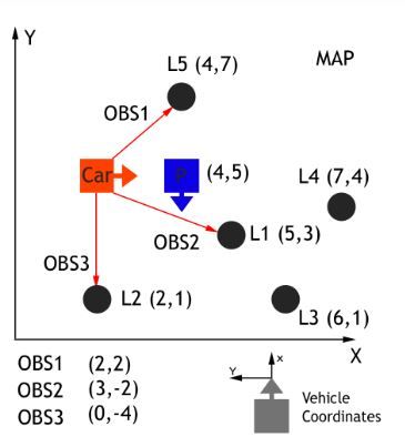
如下图所示，L1，L2，…，L5是地图(Map)中的Landmark；OBS1、OBS2、OBS3是车辆的Observation。红色方块是车辆的GroundTruth位置，蓝色方块是车辆的预测位置。

我们可以看到地图有5个LandMark，它们分别被标识为L1、L2、L3、L4、L5，并且每个LandMark都有已知的地图位置。我们需要将每个转换后的观测值TOBS1、TOBS2、TOBS3与这5个标识符中的一个相关联。其中一个直观的做法就是每个转换后的观测LandMark坐标与最近的Map LandMark相关联。

void ParticleFilter::dataAssociation(
  std::vector<LandmarkObs> predicted, 
  std::vector<LandmarkObs>& observations) {

  for (unsigned int i = 0; i < observations.size(); i++) {
    unsigned int nObs = observations.size();
    unsigned int nPred = predicted.size();
    for (unsigned int i = 0; i < nObs; i++) {  // For each observation
      double minDist = numeric_limits<double>::max();
      int mapId = -1;
      for (unsigned j = 0; j < nPred; j++) {   // For each predition.
        double xDist = observations[i].x - predicted[j].x;
        double yDist = observations[i].y - predicted[j].y;
        double distance = xDist * xDist + yDist * yDist;
        if (distance < minDist) {
          minDist = distance;
          mapId = predicted[j].id;
        }
        observations[i].id = mapId;
      }
    }
  }
}

Update Weights

完成观测LandMark坐标转换之后和地图匹配之后，就可以更新粒子的权重了。由于粒子对所有LandMark的观测都是独立的，所以粒子的总权重是所有观测LandMark的多元高斯概率密度的乘积。

\[ P(x, y) = \frac{1}{2 \pi \sigma_{x} \sigma_{y}} e^{-\left(\frac{\left(x-\mu_{x}\right)^{2}}{2 \sigma_{x}^{2}}+\frac{\left(y-\mu_{y}\right)^{2}}{2 \sigma_{y}^{2}}\right)} \]

particles[i].weight = 1.0;
for (unsigned int j = 0; j < trans_os.size(); j++) {
  double o_x, o_y, pr_x, pr_y;
  o_x = trans_os[j].x;
  o_y = trans_os[j].y;
  int asso_prediction = trans_os[j].id;

  // x,y coordinates of the prediction associated with the current observation
  // from map_landmarks
  for (unsigned int k = 0; k < predictions.size(); k++) {
    if (predictions[k].id == asso_prediction) {
      pr_x = predictions[k].x;
      pr_y = predictions[k].y;
    }
  }

  // Weight for this observation with multivariate Gaussian
  double s_x = std_landmark[0];
  double s_y = std_landmark[1];
  double obs_w = (1 / (2 * M_PI * s_x * s_y)) *
                  exp(-(pow(pr_x - o_x, 2) / (2 * pow(s_x, 2)) + 
                       (pow(pr_y - o_y, 2) / (2 * pow(s_y, 2)))));

  // Product of this obersvation weight with total observations weight
  particles[i].weight *= obs_w;
}

Resample

重采样(Resample)是从旧粒子(Old Particles)中随机抽取新粒子(New Particles)并根据其权重进行替换的过程。重采样后，具有更高权重的粒子保留的概率越大，概率越小的粒子消亡的概率越大。

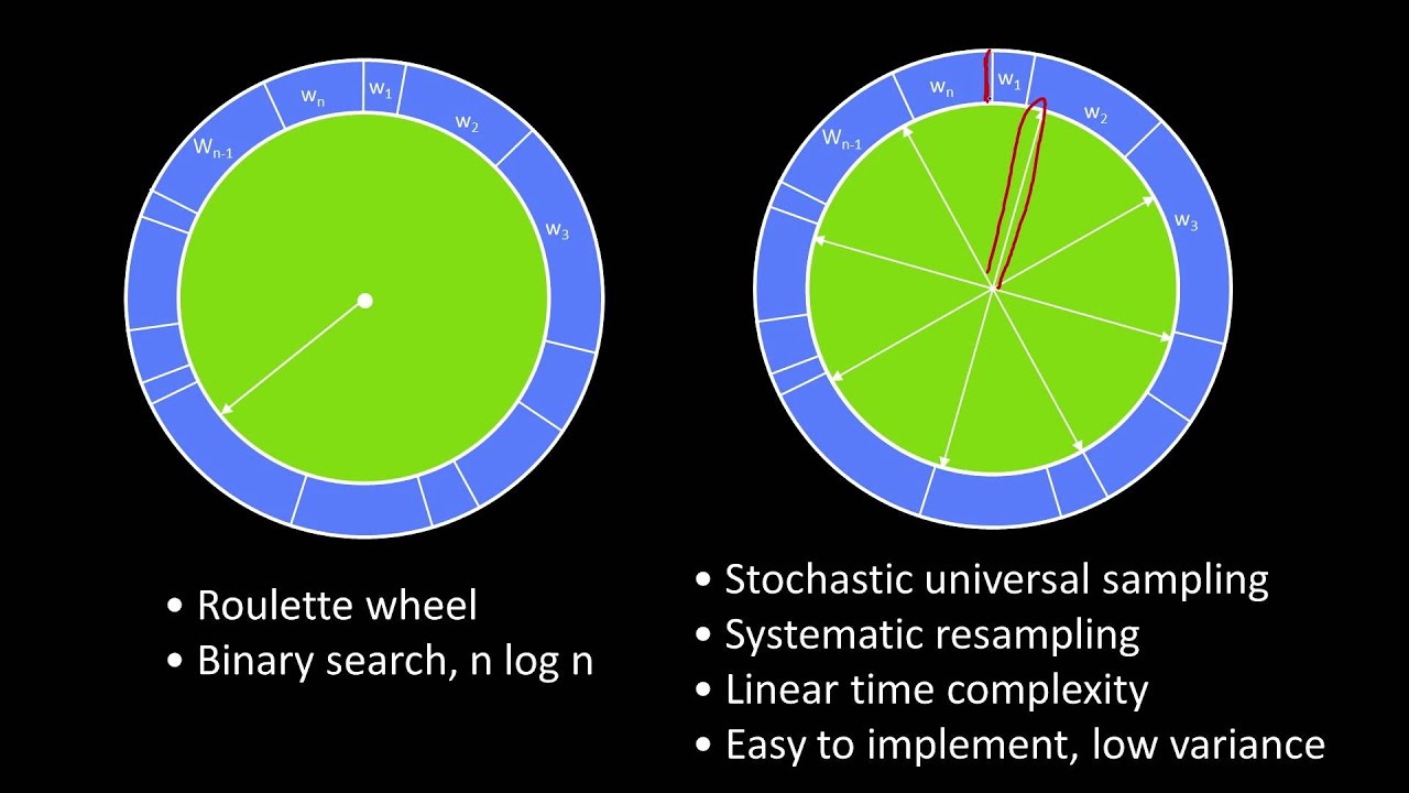
常用的Resample技术是Resampling Wheel。Resampling Wheel的算法思想如下：如下图所示的圆环，圆环的弧长正比与它的权重(即权重越大，弧长越长)。

void ParticleFilter::resample() {
  // Get weights and max weight.
  vector<double> weights;
  double maxWeight = numeric_limits<double>::min();
  for (int i = 0; i < num_particles; i++) {
    weights.push_back(particles[i].weight);
    if (particles[i].weight > maxWeight) {
      maxWeight = particles[i].weight;
    }
  }

  uniform_real_distribution<double> distDouble(0.0, maxWeight);
  uniform_int_distribution<int> distInt(0, num_particles - 1);
  int index = distInt(gen);
  double beta = 0.0;
  vector<Particle> resampledParticles;
  for (int i = 0; i < num_particles; i++) {
    beta += distDouble(gen) * 2.0;
    while (beta > weights[index]) {
      beta -= weights[index];
      index = (index + 1) % num_particles;
    }
    resampledParticles.push_back(particles[index]);
  }

  particles = resampledParticles;
}

Ref

• Kidnapped vehicle project using Particle Filters-Udacity’s Self-driving Car Nanodegree

• sohonisaurabh/CarND-Kidnapped-Vehicle-Project

• 自动驾驶定位算法(十三)-粒子滤波(Particle Filter)

• 粒子滤波（Particle filter）算法简介及MATLAB实现