计算机视觉对极几何之FEH

Overview

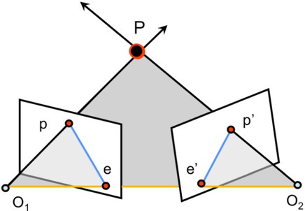
• The gray region is the epipolar plane
• The orange line is the baseline
• the two blue lines are the epipolar lines

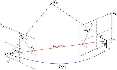
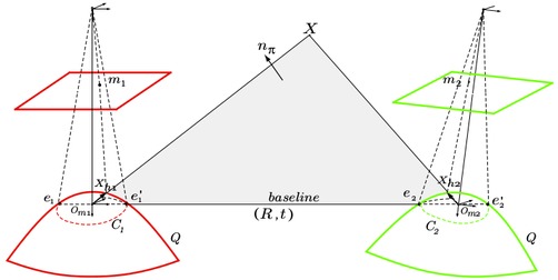
Basic Epipolar Geometry entities for pinhole cameras and panoramic camera sensors

• Fundamental Matrix \(F\)
  • maps a point in one image to a line (epiline) in the other image
  • Calculated from matching points from both the images. A minimum of 8 such points are required to find the fundamental matrix (while using 8-point algorithm). More points are preferred and use RANSAC to get a more robust result.

• Essential Matrix \(E\)

• Homography Matrix \(H\)

Foundamental Matrix (基础矩阵)

对极约束：

\[ \mathbf{p}'^T \cdot \mathbf{F} \cdot \mathbf{p} = 0 \]

其中，\(\mathbf{p}, \mathbf{p}'\) 为两个匹配 像素点坐标。

基础矩阵：

\[ \mathbf{F} = \mathbf{K}'^{-T} \mathbf{E} \mathbf{K}^{-1} = \mathbf{K}'^{-T} \mathbf{t}^\wedge \mathbf{R} \mathbf{K}^{-1} \]

或写成

\[ F = [e^\prime]_\times H_\pi \]

\(\mathbf{F}\) 的性质：

• 对其乘以 任意非零常数，对极约束依然满足（尺度等价性，up to scale）

• 奇异性约束 \(\text{rank}(\mathbf{F})=2\)
  • The fundamental matrix F may be written as \(F = [e^\prime]_\times H_\pi\) , where \(H_\pi\) is the transfer mapping from one image to another via any plane π. Furthermore, since \([e^\prime]_\times\) has rank 2 and \(H_\pi\) rank 3, \(F\) is a matrix of rank 2.
  • 两个相机内参矩阵和旋转矩阵R都是满秩矩阵（可逆矩阵），\(t^\wedge\) 是一个秩为2的矩阵，同样，矩阵乘以可逆矩阵秩不变，因为可逆矩阵可以表示为初等矩阵的乘积，而初等变换不改变矩阵的秩（左乘-行变换，右乘-列变换）。
• 具有 7个自由度
  • a 3×3 homogeneous matrix has eight independent ratios (there are nine elements, and the common scaling is not significant)
  • F also satisfies the constraint det F = 0 which removes one degree of freedom.

\(\mathbf{F}\) 与 极线和极点 的关系：

\[ \mathbf{l}' = \mathbf{F} \cdot \mathbf{p} \]

\[ \mathbf{l} = \mathbf{F}^T \cdot \mathbf{p}' \]

\[ \mathbf{F} \cdot \mathbf{e} = \mathbf{F}^T \cdot \mathbf{e}' = 0 \]

Foundamental Matrix Estimation

类似于下面 \(\mathbf{E}\) 的估计

• 归一化8点法（Eight-Point Algorithm）
• 7点法
• 6点法

Essential Matrix (本质矩阵)

对极约束：

\[ {\mathbf{p}'}^T \cdot \mathbf{E} \cdot \mathbf{p} = 0 \]

其中，\(\mathbf{p}, \mathbf{p}'\) 为两个匹配像素点的 归一化平面坐标。

本质矩阵：

\[ \mathbf{E} = \mathbf{t}^\wedge \mathbf{R} = \mathbf{K}'^{T} \mathbf{F} \mathbf{K} \\[2ex] \]

\(\mathbf{E}\) 的性质：

• A 3×3 matrix is an essential matrix if and only if two of its singular values are equal, and the third is zero

• 对其乘以 任意非零常数，对极约束依然满足 尺度等价性 (up to scale)

• 奇异性约束 \(\text{rank}(\mathbf{E})=2\)
  • \(\text{rank}(\mathbf{t^\wedge})=2\)；\(R\)为可逆矩阵，可逆矩阵不改变矩阵的秩
  • 根据 \(\mathbf{E} = \mathbf{t}^\wedge \mathbf{R}\)，\(\mathbf{E}\) 的奇异值必定是 \([\sigma, \sigma, 0]^T\) 的形式
• 具有 5个自由度
  • 平移旋转共6个自由度 - 尺度等价性
  • both the rotation matrix R and the translation t have three degrees of freedom, but there is an overall scale ambiguity – like the fundamental matrix, the essential matrix is a homogeneous quantity

\(\mathbf{E}\) 与 极线和极点 的关系：

\[ \mathbf{l}' = \mathbf{E} \cdot \mathbf{p} \]

\[ \mathbf{l} = \mathbf{E}^T \cdot \mathbf{p}' \]

\[ \mathbf{E} \cdot \mathbf{e} = \mathbf{E}^T \cdot \mathbf{e}' = 0 \]

Essential Matrix Estimation

• 5点法（最少5对点求解）
• 8点法（Eight-Point Algorithm）
  • 8点法成功的关键是在构造解的方程之前应对输入的数据认真进行适当的 归一化，图像点的一个简单变换(平移或变尺度)将使这个问题的条件极大地改善，从而提高结果的稳定性

矩阵形式：

\[ \begin{bmatrix} x' & y' & 1 \end{bmatrix} \cdot \begin{bmatrix} e_{1} & e_{2} & e_{3} \\ e_{4} & e_{5} & e_{6} \\ e_{7} & e_{8} & e_{9} \end{bmatrix} \cdot \begin{bmatrix} x \\ y \\ 1 \end{bmatrix} = 0 \]

矩阵 \(\mathbf{E}\) 展开，写成向量形式 \(\mathbf{e}\)，并把所有点（n对点，n>=8）放到一个方程中，齐次线性方程组 如下：

\[ \begin{bmatrix} x'^1x^1 & x'^1y^1 & x'^1 & y'^1x^1 & y'^1y^1 & y'^1 & x^1 & y^1 & 1 \\ x'^2x^2 & x'^2y^2 & x'^2 & y'^2x^2 & y'^2y^2 & y'^2 & x^2 & y^2 & 1 \\ \vdots & \vdots & \vdots & \vdots & \vdots & \vdots & \vdots & \vdots & \vdots \\ x'^nx^n & x'^ny^n & x'^n & y'^nx^n & y'^ny^n & y'^n & x^n & y^n & 1 \\ \end{bmatrix} \cdot \begin{bmatrix} e_{1} \\ e_{2} \\ e_{3} \\ e_{4} \\ e_{5} \\ e_{6} \\ e_{7} \\ e_{8} \\ e_{9} \end{bmatrix} = 0 \]

即（the essential matrix lying in the null space of this matrix A）

\[ \mathbf{A} \cdot \mathbf{e} = \mathbf{0} \quad s.t. \quad \mathbf{A} \in \mathbb{R}^{n \times 9}, n \geq 8 \]

对上式 求解 最小二乘解（尺度等价性）

\[ \min_{\mathbf{e}} \|\mathbf{A} \cdot \mathbf{e}\|^2 \quad s.t. \quad \|\mathbf{e}\| = 1 \quad \text{or} \quad {\|\mathbf{E}\|}_F = 1 \]

SVD分解 \(\mathbf{A}\)（或者 EVD分解 \(\mathbf{A}^T \mathbf{A}\)）

\[ \text{SVD}(\mathbf{A}) = \mathbf{U} \mathbf{D} \mathbf{V}^T \]

\(\mathbf{e}\) 正比于 \(\mathbf{V}\) 的最后一列，得到 \(\mathbf{E}\)

根据 奇异性约束 \(\text{rank}(\mathbf{E})=2\)，再 SVD分解 \(\mathbf{E}\)

\[ \text{SVD}(\mathbf{E}) = \mathbf{U}_E \mathbf{D}_E \mathbf{V}_E^T \]

求出的 \(\mathbf{E}\) 可能不满足其内在性质（奇异值是 \([\sigma, \sigma, 0]^T\) 的形式），此时对 \(\mathbf{D}_E\) 进行调整，假设 \(\mathbf{D}_E = \text{diag}(\sigma_1, \sigma_2, \sigma_3)\) 且 \(\sigma_1 \geq \sigma_2 \geq \sigma_3\)，则令

\[ \mathbf{D}_E' = \text{diag}(\frac{\sigma_1+\sigma_2}{2}, \frac{\sigma_1+\sigma_2}{2}, 0) \]

或者，更简单的（尺度等价性）

\[ \mathbf{D}_E' = \text{diag}(1, 1, 0) \]

最后，\(\mathbf{E}\) 矩阵的正确估计为

\[ \mathbf{E}' = \mathbf{U}_E \mathbf{D}_E' \mathbf{V}_E^T \]

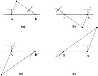
Rotation and translation from E

The four possible solutions for calibrated reconstruction from E

• Between the left and right sides there is a baseline reversal
• Between the top and bottom rows camera B rotates 180 about the baseline
• only in (a) is the reconstructed point in front of both cameras

Suppose that the SVD of \(E\) is

\[ \text{SVD}(E) = U \text{diag}(1, 1, 0) V^T \]

there are (ignoring signs) two possible factorizations \(E = t^\wedge R = SR\) as follows

\[ \begin{aligned} t^\wedge &= UZU^T \quad or \quad U(-Z)U^T \\[2ex] R &= UWV^T \quad or \quad UW^TV^T \end{aligned} \]

where

\[ \begin{aligned} W &= \begin{bmatrix} 0 & -1 & 0 \\ 1 & 0 & 0 \\ 0 & 0 & 1 \end{bmatrix} = R_z(\frac{\pi}{2}) \\[3ex] Z &= \begin{bmatrix} 0 & 1 & 0 \\ -1 & 0 & 0 \\ 0 & 0 & 0 \end{bmatrix} = \text{diag}(1, 1, 0) \cdot W \end{aligned} \]

• \(W\) is orthogonal
• \(Z\) is skew-symmetric
• also we can get \(t\) with \(t = U(0,0,1)^T = \mathbf{u}_3\), the last column of \(U\)

Rt恢复示例代码 e2rt.cpp：

Matrix3d E;
E << -0.0203618550523477,   -0.4007110038118445,  -0.03324074249824097,
      0.3939270778216369,   -0.03506401846698079,  0.5857110303721015,
     -0.006788487241438284, -0.5815434272915686,  -0.01438258684486258;

cout << "E = \n" << E << endl;

// SVD and fix sigular values
JacobiSVD<MatrixXd> svd(E, ComputeThinU | ComputeThinV);
Matrix3d m3U = svd.matrixU();
Matrix3d m3V = svd.matrixV();
Vector3d v3S = svd.singularValues();

double temp = (v3S[0]+v3S[1])/2;
Matrix3d m3S(Vector3d(temp, temp, 0).asDiagonal());

Eigen::Matrix3d m3R_z_p = Eigen::AngleAxisd( M_PI/2, Eigen::Vector3d(0,0,1)).toRotationMatrix();
Eigen::Matrix3d m3R_z_n = Eigen::AngleAxisd(-M_PI/2, Eigen::Vector3d(0,0,1)).toRotationMatrix();
cout << "m3R_z_p = \n" << m3R_z_p << endl;
cout << "m3R_z_n = \n" << m3R_z_n << endl;

// set t1, t2, R1, R2
Matrix3d t_wedge1;
Matrix3d t_wedge2;
t_wedge1 = m3U * m3R_z_p * m3S * m3U.transpose();
t_wedge2 = m3U * m3R_z_n * m3S * m3U.transpose();

Matrix3d R1;
Matrix3d R2;
R1 = m3U * m3R_z_p.transpose() * m3V.transpose();
R2 = m3U * m3R_z_n.transpose() * m3V.transpose();

cout << "R1 = \n" << R1 << endl;
cout << "R2 = \n" << R2 << endl;
cout << "t1 = \n" << Sophus::SO3::vee(t_wedge1) << endl;
cout << "t2 = \n" << Sophus::SO3::vee(t_wedge2) << endl;

// check t^R=E up to scale
Matrix3d tR = t_wedge1 * R1;
cout << "t^R = \n" << tR << endl;

DecomposeE in ORB-SLAM2

void Initializer::DecomposeE(const cv::Mat &E, cv::Mat &R1, cv::Mat &R2, cv::Mat &t) {
    cv::Mat u,w,vt;
    cv::SVD::compute(E,w,u,vt);

    u.col(2).copyTo(t);
    t=t/cv::norm(t);

    cv::Mat W(3,3,CV_32F,cv::Scalar(0));
    W.at<float>(0,1)=-1;
    W.at<float>(1,0)=1;
    W.at<float>(2,2)=1;

    R1 = u*W*vt;
    if(cv::determinant(R1)<0)
        R1=-R1;

    R2 = u*W.t()*vt;
    if(cv::determinant(R2)<0)
        R2=-R2;
}

CheckRT in ORB-SLAM2

Homography Matrix (单应性矩阵)

• For planar surfaces, 3D to 2D perspective projection reduces to a 2D to 2D transformation
• 从零开始一起学习SLAM | 神奇的单应矩阵

设图像 \(I_1\) 和 图像 \(I_2\) 有一对匹配好的特征点 \(p_1\) 和 \(p_2\)。这个特征点落在平面 \(P\) 上，设这个平面满足方程：

\[ \mathbf{n}^T \mathbf{P} + d = 0 \]

单应性矩阵 通常描述处于 共同平面 上的一些点在 两张图像之间的变换关系：

\[ \begin{aligned} \mathbf{p}_2 &\simeq \mathbf{K}_2 \left(\mathbf{R} \mathbf{P} + \mathbf{t} \right) \\ &\simeq \mathbf{K}_2 \left(\mathbf{R} \mathbf{P} + \mathbf{t} \cdot\left(-\frac{\mathbf{n}^{T} \mathbf{P}}{\mathbf{d}}\right)\right) \\ &\simeq \mathbf{K}_2 \left(\mathbf{R} - \frac{\mathbf{t} \mathbf{n}^T}{d}\right) \mathbf{P} \\ &\simeq \mathbf{K}_2 \left(\mathbf{R} - \frac{\mathbf{t} \mathbf{n}^T}{d}\right) \mathbf{K}_1^{-1} \mathbf{p}_1 \\ &\simeq \mathbf{H} \cdot \mathbf{p}_1 \end{aligned} \]

单应性矩阵：

\[ \mathbf{H} = \mathbf{K}_2 (\mathbf{R} - \frac{\mathbf{t} \mathbf{n}^T}{d}) \mathbf{K}_1^{-1} \]

\(\mathbf{H}\) 的性质：

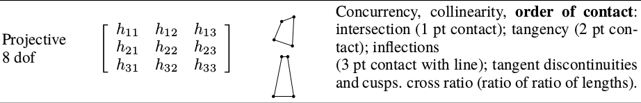
• 具有 8个自由度
  • 尺度等价性: 9 -1 = 8

Homography Estimation

矩阵形式：

\[ \begin{bmatrix} x' \\ y' \\ 1 \end{bmatrix} = \begin{bmatrix} h_{11} & h_{12} & h_{13} \\ h_{21} & h_{22} & h_{23} \\ h_{31} & h_{32} & h_{33} \end{bmatrix} \cdot \begin{bmatrix} x \\ y \\ 1 \end{bmatrix} \]

方程形式（两个约束条件）：

\[ x' = \frac { h_{11}x + h_{12}y + h_{13} } { h_{31}x + h_{32}y + h_{33} } \\[2ex] y' = \frac { h_{21}x + h_{22}y + h_{23} } { h_{31}x + h_{32}y + h_{33} } \]

因为上式使用的是齐次坐标，所以我们可以 对 所有的 \(h_{ij}\) 乘以 任意的非0因子 而不会改变方程。

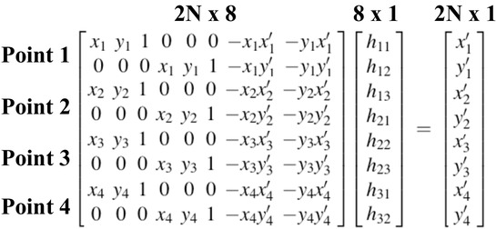
归一化4点法

• 因此， \(\mathbf{H}\) 具有 8个自由度，最少通过 4对匹配点（不能出现3点共线） 算出。

• 实际中，通过 \(h_{33}=1\) 或 \(\|\mathbf{H}\|_F=1\) 两种方法 使 \(\mathbf{H}\) 具有 8自由度。

cont 1: H元素h33=1

线性方程：

\[ \mathbf{A} \cdot \mathbf{h} = \mathbf{b} \]

求解：

\[ \mathbf{A}^T \mathbf{A} \cdot \mathbf{h} = \mathbf{A}^T \mathbf{b} \]

所以

\[ \mathbf{h} = (\mathbf{A}^T \mathbf{A})^{-1} \mathbf{A}^T \mathbf{b} \]

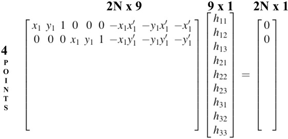
cont 2: H的F范数|H|=1

线性方程：

\[ \mathbf{A} \cdot \mathbf{h} = \mathbf{0} \]

求解：

\[ \mathbf{A}^T \mathbf{A} \cdot \mathbf{h} = \mathbf{0} \]

对上式 求解 最小二乘解（尺度等价性）

\[ \min_{\mathbf{h}} \|(\mathbf{A}^T \mathbf{A}) \cdot \mathbf{h}\|^2 \quad s.t. \quad \|\mathbf{h}\| = 1 \quad \text{or} \quad {\|\mathbf{H}\|}_F = 1 \]

SVD分解 或 特征值分解

\[ \text{SVD}(\mathbf{A}^T \mathbf{A}) = \mathbf{U} \boldsymbol{\Sigma} \mathbf{U}^T \]

最后 \(\mathbf{h}\) 为 \(\boldsymbol{\Sigma}\) 中 最小特征值 对应的 \(\mathbf{U}\) 中的列向量（单位特征向量）；如果只用4对匹配点，那个特征值为0。

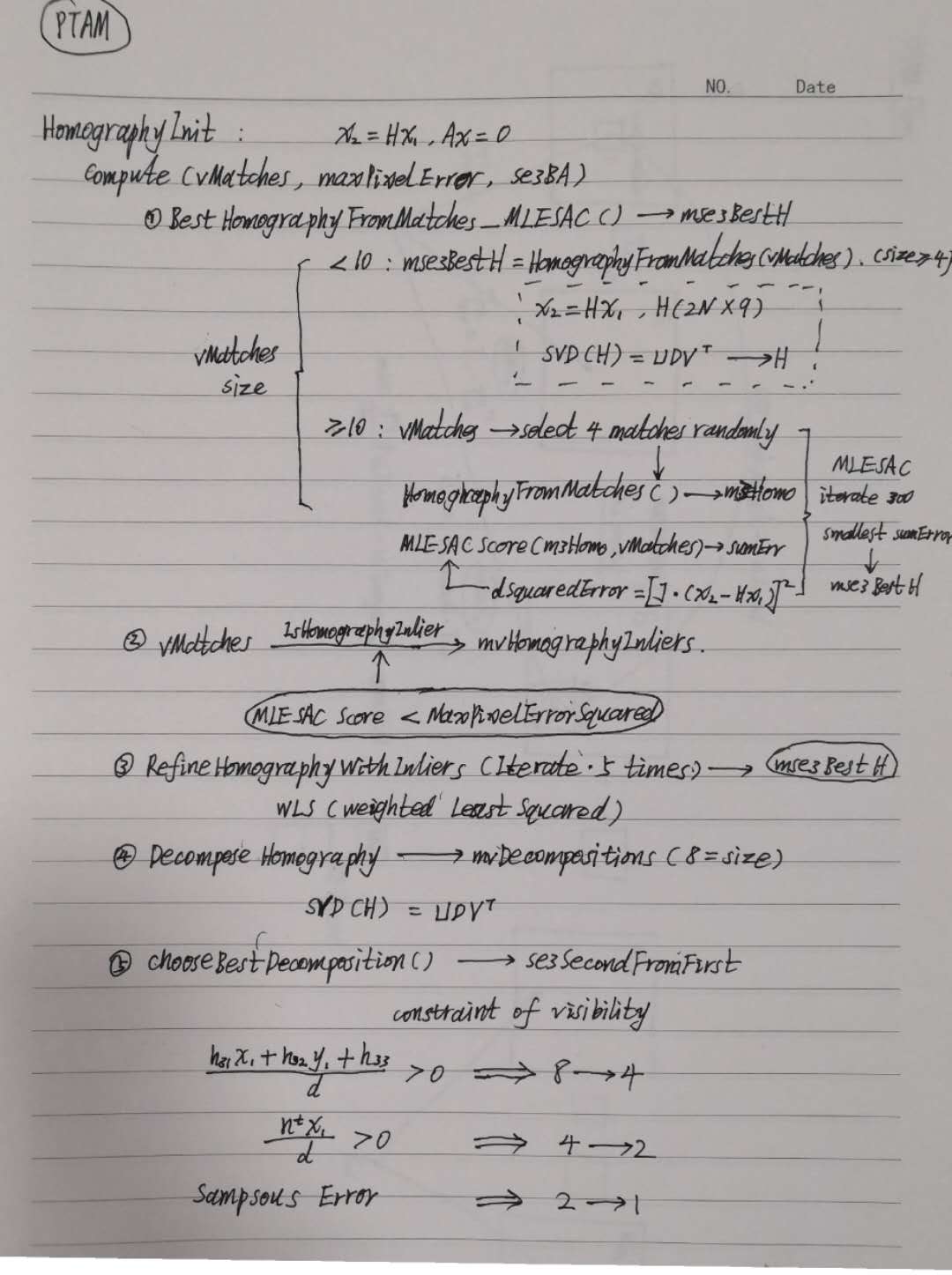
H in PTAM

• 相关代码

单应性矩阵的计算

Matrix<3> HomographyInit::HomographyFromMatches(vector<HomographyMatch> vMatches)
{
    unsigned int nPoints = vMatches.size();
    assert(nPoints >= 4);
    int nRows = 2*nPoints;
    if(nRows < 9)
        nRows = 9;
    Matrix<> m2Nx9(nRows, 9);
    for(unsigned int n=0; n<nPoints; n++)
    {
        double u = vMatches[n].v2CamPlaneSecond[0];
        double v = vMatches[n].v2CamPlaneSecond[1];

        double x = vMatches[n].v2CamPlaneFirst[0];
        double y = vMatches[n].v2CamPlaneFirst[1];

        // [u v]T = H [x y]T
        m2Nx9[n*2+0][0] = x;
        m2Nx9[n*2+0][1] = y;
        m2Nx9[n*2+0][2] = 1;
        m2Nx9[n*2+0][3] = 0;
        m2Nx9[n*2+0][4] = 0;
        m2Nx9[n*2+0][5] = 0;
        m2Nx9[n*2+0][6] = -x*u;
        m2Nx9[n*2+0][7] = -y*u;
        m2Nx9[n*2+0][8] = -u;

        m2Nx9[n*2+1][0] = 0;
        m2Nx9[n*2+1][1] = 0;
        m2Nx9[n*2+1][2] = 0;
        m2Nx9[n*2+1][3] = x;
        m2Nx9[n*2+1][4] = y;
        m2Nx9[n*2+1][5] = 1;
        m2Nx9[n*2+1][6] = -x*v;
        m2Nx9[n*2+1][7] = -y*v;
        m2Nx9[n*2+1][8] = -v;
    }

    if(nRows == 9)
        for(int i=0; i<9; i++)  // Zero the last row of the matrix,
            m2Nx9[8][i] = 0.0;  // TooN SVD leaves out the null-space otherwise

    // The right null-space of the matrix gives the homography...
    SVD<> svdHomography(m2Nx9);
    Vector<9> vH = svdHomography.get_VT()[8];
    Matrix<3> m3Homography;
    m3Homography[0] = vH.slice<0,3>();
    m3Homography[1] = vH.slice<3,3>();
    m3Homography[2] = vH.slice<6,3>();
    return m3Homography;
};

Rotation and translation from H

• Motion and structure from motion in a piecewise planar environment

手写笔记

Degenerate Case (退化情况)

The computation of the two-view geometry requires that the matches originate from a 3D scene and that the motion is more than a pure rotation. If the observed scene is planar, the fundamental matrix is only determined up to three degrees of freedom. The same is true when the camera motion is a pure rotation. In this last case -only having one center of projection- depth can not be observed. In the absence of noise the detection of these degenerate cases would not be too hard. Starting from real -and thus noisy- data, the problem is much harder since the remaining degrees of freedom in the equations are then determined by noise. Different models are evaluated. In this case the fundamental matrix (corresponding to a 3D scene and more than a pure rotation), a general homography (corresponding to a planar scene) and a rotation-induced homography are computed. Selecting the model with the smallest residual would always yield the most general model.

• If the scene is planar, nearly planar or there is low parallax, it can be explained by a homography.

• a non-planar scene with enough parallax can only be explained by the fundamental matrix, but a homography can also be found explaining a subset of the matches if they lie on a plane or they have low parallax (they are far away)

Reference

• Epipolar Geometry and the Fundamental Matrix in MVG (Chapter 9)
• 《视觉SLAM十四讲》