StereoScan(libVISO2) 学习笔记

Overview

LIBVISO2 (Library for Visual Odometry 2) is a very fast cross-platfrom (Linux, Windows) C++ library with MATLAB wrappers for computing the 6 DOF motion of a moving mono/stereo camera.

• The stereo version is based on minimizing the reprojection error of sparse feature matches and is rather general (no motion model or setup restrictions except that the input images must be rectified and calibration parameters are known).

• The monocular version is still very experimental and uses the 8-point algorithm for fundamental matrix estimation. It further assumes that the camera is moving at a known and fixed height over ground (for estimating the scale). Due to the 8 correspondences needed for the 8-point algorithm, many more RANSAC samples need to be drawn, which makes the monocular algorithm slower than the stereo algorithm, for which 3 correspondences are sufficent to estimate parameters.

Paper & Code

• papers: StereoScan: Dense 3D Reconstruction in Real-time
• code: cggos/viso2_cg

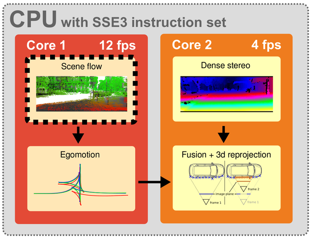
Scen Flow

Feature Matching

Feature Detection

Blob/Corner Detector:

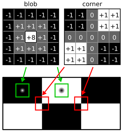
• filter the input images with 5×5 blob and corner masks
  
• employ non-maximum- and non-minimum-suppression on the filtered images, resulting in feature candidates

Feature Descriptor:

The descriptor concatenates Sobel filter responses using the layout given in below:

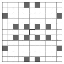
simply compare 11 × 11 block windows of horizontal and vertical Sobel filter responses to each other by using the sum of absolute differences (SAD) error metric; to speed-up matching, we quantize the Sobel responses to 8 bits and sum the differences over a sparse set of 16 locations instead of summing over the whole block window; since the SAD of 16 bytes can be computed efficiently using a single SSE instruction we only need two calls (for horizontal + vertical Sobel responses) in order to evaluate this error metric

• 16 locations within 11 × 11 block window
• 32 bytes per descriptor
• Efficient Sum-of-Absolute-Differences (SAD) via SIMD

Circle Match

Starting from all feature candidates in the current left image, we find the best match in the previous left image within a M × M search window, next in the previous right image, the current right image and last in the current left image again.

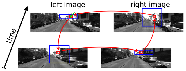
A ’circle match’ gets accepted, if the last feature coincides with the first feature.

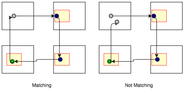
• Detect interest points using non-maximum-suppression
• Match 4 images in a ’space-time’ circle
• make use of the epipolar constraint using an error tolerance of 1 pixel when matching between the left and right images
• Accept if last feature coincides with first feature

Fast Feature Matching

• 1st: Match a sparse set of interest points within each class
• Build statistics over likely displacements within each bin
• Use this statistics for speeding up 2nd matching stage
• Rejection outliers (Delaunay triangulation)

Egomotion Estimation

Features Bucketing

keeps only max_features per bucket, where the domain is split into buckets of size (bucket_width,bucket_height).

• reduce the number of features (in practice we retain between 200 and 500 features)
• spread them uniformly over the image domain

3D Points Calcuation

• disparity

\[ d = max(u_l - u_r, 0.001) \]

• Stereo Baseline

\[ B = stereomodel.baseline \]

• 3d points

\[ \begin{aligned} \begin{cases} Z = \frac{f \cdot B}{d} \\ X = (u-c_u) \cdot \frac{B}{d} \\ Y = (v-c_v) \cdot \frac{B}{d} \end{cases} \end{aligned} \]

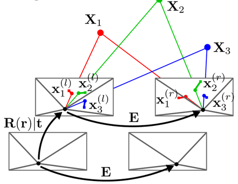
Projection Model

Assuming squared pixels and zero skew, the reprojection into the current image is given by

\[ \begin{bmatrix} u_c \\ v_c \\ 1 \end{bmatrix} = \begin{bmatrix} f & 0 & c_u \\ 0 & f & c_v \\ 0 & 0 & 1 \end{bmatrix} \begin{bmatrix} (\mathbf{R}(r) \quad \mathbf{t}) \left( \begin{array}{cccc} X_p \\ Y_p \\ Z_p \end{array} \right) - \left( \begin{array}{cccc} s \\ 0 \\ 0 \end{array} \right) \end{bmatrix} \]

• homogeneous image coordinates \((u_c \quad v_c \quad 1 )^T\)
• focal length \(f\)
• principal point \((c_u, c_v )\)
• rotation matrix \(\mathbf{R}(r) = \mathbf{R}_x (r_x ) \mathbf{R}_y(r_y) \mathbf{R}_z(r_z)\)
• translation vector \(\mathbf{t} = (t_x \quad t_y \quad t_z )\)
• 3d point coordinates \(\mathbf{P} = (X_p \quad Y_p \quad Z_p)\)
• shift \(s = 0\) (left image), \(s = baseline\) (right image)

Minimize Reprojection Errors

Compute the camera motion by minimizing the sum of reprojection errors iteratly by using Gauss-Newton optimization and RANSAC.

• reprojection errors

\[ \begin{aligned} \min_{\beta} {\| r(\beta) \|}^2 =& \sum_{i=1}^N {\| p_i^{(l)} - p_i'^{(l)} \|}^2 + {\| p_i^{(r)} - p_i'^{(r)} \|}^2\\ =& \sum_{i=1}^N {\| p_i^{(l)} - \pi^{(l)}(P_i; R,t) \|}^2 + {\| p_i^{(r)} - \pi^{(r)}(P_i; R,t) \|}^2 \\ =& \sum_{i=1}^3 (u_i^l-u^l)^2 + (v_i^l-v^l)^2 + (u_i^r-u^r)^2 + (v_i^r-v^r)^2 \end{aligned} \]

• errors vector

\[ \begin{aligned} r(\beta) =& (r_0, r_1, r_2, \cdots, r_{N}) \\ =& ( r_{u_{0l}}, r_{v_{0l}}, r_{u_{0r}}, r_{v_{0r}}, r_{u_{1l}}, r_{v_{1l}}, r_{u_{1r}}, r_{v_{1r}}, r_{u_{2l}}, r_{v_{2l}}, r_{u_{2r}}, r_{v_{2r}} ) \in \mathbb{R}^{4 \times N} \quad \text{s.t.} \quad N = 3 \end{aligned} \]

• Optimization parameters vector

\[ \beta = (r_x, r_y, r_z, t_x, t_y, t_z) \in \mathbb{R}^{6 \times 1} \]

• Jocobians Matrix

\[ J_{(4 \times N) \times 6} = \frac{\partial{r(\beta)}}{\partial{\beta}} \quad \text{s.t.} \quad N = 3 \]

• Parameter iteration

\[ \beta_i = \beta_{i-1} - (J^TJ)^{-1} \cdot J^T r(\beta_{i-1}) \]

Jacobian Matrix Compute

\[ \begin{aligned} J_{2 \times 6} =& \frac{\partial(r_{u_{0l}}, r_{v_{0l}})}{\partial \beta} \\ =& J_1 \cdot J_2 \cdot J_3 \\ =& \frac{ \partial{ (p^{(l)} - p'^{(l)}) } }{ \partial{ p'^{(l)} } } \cdot \frac{ \partial{ p'^{(l)} } }{ \partial{P'^{(l)}} } \cdot \frac{ \partial{ P'^{(l)} } }{ \partial \beta} \\ =& I \cdot \begin{bmatrix} \frac{f}{Z'} & 0 & -\frac{f}{Z'^2} X' \\ 0 & \frac{f}{Z'} & -\frac{f}{Z'^2} Y' \end{bmatrix} \cdot \begin{bmatrix} \frac{\partial \mathbf R}{\partial r_x} X_p & \frac{\partial \mathbf R}{\partial r_y} X_p & \frac{\partial \mathbf R}{\partial r_z} X_p & 1 & 0 & 0 \\ \frac{\partial \mathbf R}{\partial r_x} Y_p & \frac{\partial \mathbf R}{\partial r_y} Y_p & \frac{\partial \mathbf R}{\partial r_z} Y_p & 0 & 1 & 0 \\ \frac{\partial \mathbf R}{\partial r_x} Z_p & \frac{\partial \mathbf R}{\partial r_y} Z_p & \frac{\partial \mathbf R}{\partial r_z} Z_p & 0 & 0 & 1 \end{bmatrix} \end{aligned} \]

Kalman Filter

refine the obtained velocity estimates by means of a Kalman filter(constant acceleration model)

Stereo Matching

Stereo matching stage takes the output of the feature matching stage and builds a disparity map for each frame. In this paper, the disparity map is built with a free library called ELAS. ELAS is a novel approach to binocular stereo for fast matching of high resolution imagery.

3D Reconstruction

The simplest method to point-based 3d reconstructions map all valid pixels to 3d and projects them into a common coordinate system using the egomotion matrix.