Mesh Texturing in a Nutshell (Let There Be Color)
Last updated on November 26, 2023 pm
[TOC]
Overview
- code (forked): https://github.com/cggos/mvs-texturing
- paper: Let There Be Color! Large-Scale Texturing of 3D Reconstructions
- video: https://www.youtube.com/watch?v=Ie-qLJdmlLI
1. Texture Views
1 | |
2. Mesh --> MeshInfo
1 | |
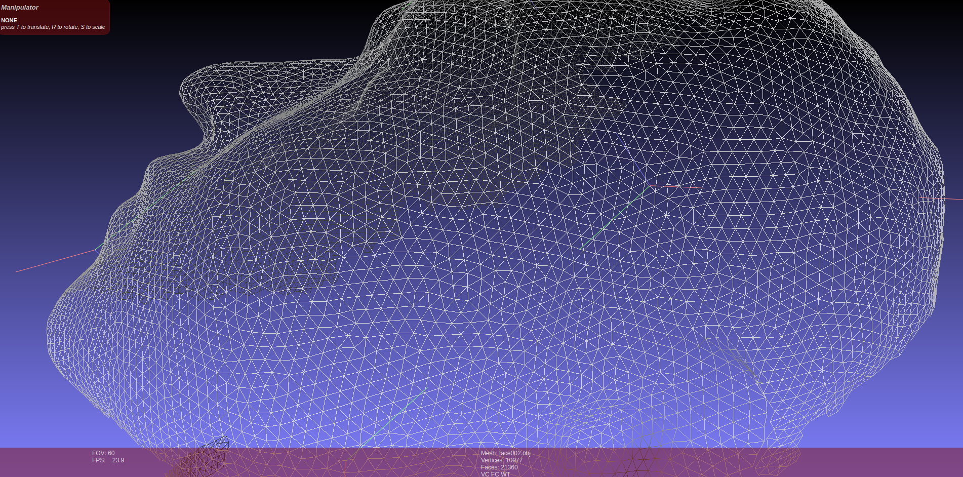
Check Mesh
1 | |
- Ensure face and vertex normals
Init MeshInfo
1 | |
Create VertexInfo
Add faces to their three vertices
Update VertexInfo
Classify each vertex and compute adjacenty info
- Build new, temporary adjacent faces representation
AdjacentFaceList adj_tempfor ordering
digraph { face_id [color=green]; front_vid [color=blue]; back_vid [color=blue];
AdjFaceTmp->face_id AdjFaceTmp->front_vid AdjFaceTmp->back_vid }graph { layout=twopi; node [shape=circle];
v0 [color="red"]; v1 [color="blue"]; v2 [color="blue"];
v0--v1 [color=green]; v0--v2 [color=green]; v0--v3; v0--v4; v1--v2 [color=green]; v3--v2; v3--v4; v1--v4;
overlap=false; }Sort adjacent faces by chaining them
1
AdjacentFaceList adj_sorted;update
VertexInfo
digraph { vclass; verts [color=blue]; faces [color=green];
vinfo->vclass; vinfo->verts; vinfo->faces; }3. Mesh + MeshInfo
--> Adjacency Graph (UniGraph)
1 | |
对于每个 face,将mesh中与其每条 edge 邻接的 face 存入
adj_faces;将当前 face 与 adj_faces 中每个
face 建立 edge,构建 UniGraph 。
graph { node [shape=circle];
f0--f1; f1--f2; f0--f3; f3--f4; f1--f4;
overlap=false; }4. View Selection --> Best View Label 😄
1 | |
Calculate DataCosts
Calculates the data costs for each face and texture view combination, if the face is visible within the texture view.
1 | |
Calculate
FaceProjectionInfo
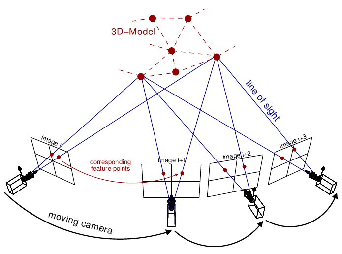
1 | |
PostProcess Face Infos
create hist_qualities::Histogram using
info.quality, and get the upper_bound when
percentile=0.995
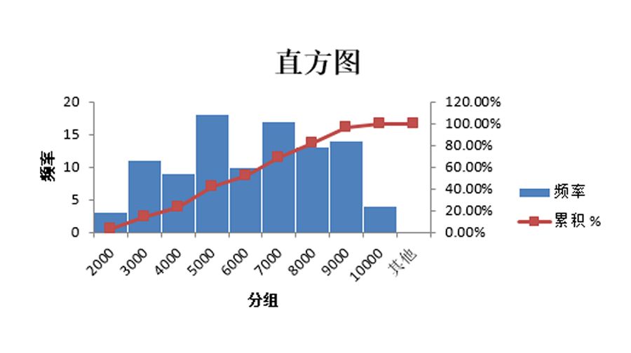
compute data cost
- gmi
- area
1 | |
| DataCost | face0 | face1 | ... | faceN |
|---|---|---|---|---|
| view0 | ||||
| view1 | ||||
| ... | ||||
| viewN |
View Selection
Data Association
Graph
mapmap::Graph<cost_t>
LabelSet
mapmap::LabelSet<cost_t, simd_w>
| view id | face0 | face1 | ... | faceN |
|---|---|---|---|---|
| view0 | ||||
| view1 | ||||
| ... | ||||
| viewN |
Unaries
1 | |
| face_id | label_set | costs | |
|---|---|---|---|
| unary0 | |||
| unary1 | |||
| ... | |||
| unaryN |
Pairwise
1 | |
MAP-MRF 🚩
1 | |
The aim is to find a labeling for X that produces the lowest energy.
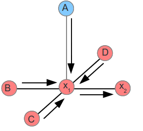
pairwise MRFs

- the filled-in circles: the observed nodes \(Y_i\) (face)
- the empty circles: the "hidden" nodes \(X_i\) (view label)
MAP --> Minimum Energy
energy/cost function:
\[ \text{energy} (Y, X) = \sum_{i} \text{DataCost} (y_i, x_i) + \sum_{j = \text{neighbours of i}} \text{SmoothnessCost} (x_i, x_j) \]
Tree MRFs via DP

LBP
by OpenMVS
5. Create Texture Atlases 😄
1 | |
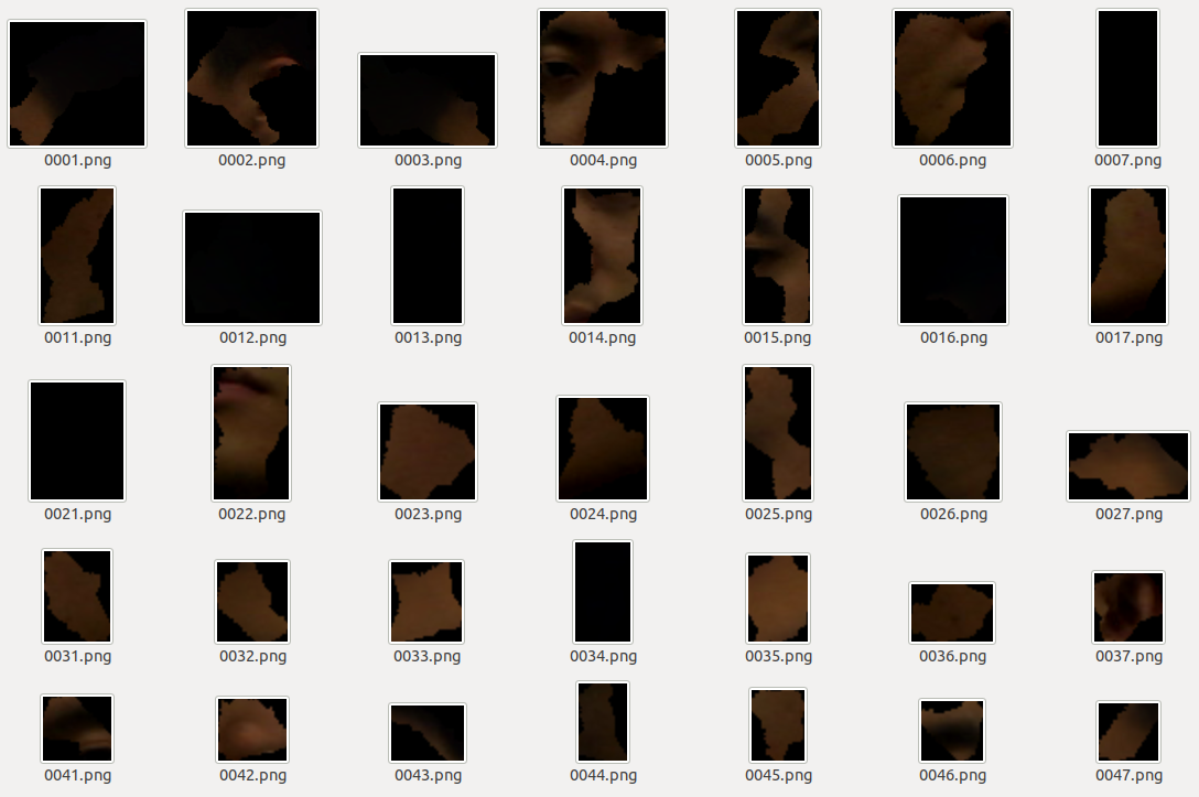
Generate Texture Patches
Generates texture patches using the graph to determine adjacent faces with the same label.
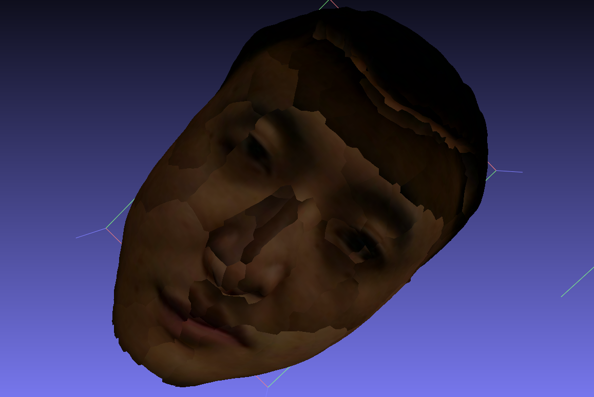
Global / Local Seam Levelling 🚩
- paper: Seamless Mosaicing of Image-Based Texture Maps

without seam levelling
Texture Atlases
generate TextureAtlas from all of
TexturePatch

6. Mesh + Texture --> Obj Model
1 | |
- .obj
- .mtl
- .png

网格UV展开
上述纹理重建属于 计算机视觉 的内容,本节是其逆过程,属于 计算机图形学 的内容。
- http://geometryhub.net/notes/uvunfold

Reference
- UV的概念及作用
- 【Let It Be Color!——3D重建之纹理重建】02-基于映射的纹理重建算法(上)
- https://github.com/tyluann/3DTexture
- https://zhuanlan.zhihu.com/p/44424934