Multi-Sensor Fusion: LiDAR and Radar fusion based on UKF

[TOC]

Overview

• code: cggos/lidar_radar_fusion_ekf_ukf

EKF v.s. UKF v.s. PF

• EKF: 通过 泰勒分解将模型线性化 求出预测模型的概率均值和方差

  • 线性、高斯
  • 对于非线性问题， EKF除了计算量大，还有线性误差的影响

• UKF: 通过 不敏变换 来求出预测模型的均值和方差

  • 非线性、高斯
  • UKF生成了一些点，来近似非线性，由这些点来决定实际x和P的取值范围
    • 跟 粒子滤波器(PF) 不同的是，UKF里Sigma点的生成并没有概率的问题

• PF: 非线性、非高斯

UKF v.s. CKF

UKF、CKF：同属点估计方法，不是说高斯分布非线性转移以后不再是高斯分布，所以kf无法继续迭代么。那么它俩就不管了，在转移之前取一坨点近似一个分布，直接通过数学模型算出转移以后的一坨点（代x算fx），然后通过一些“科学方法”去估计转移以后的那一坨点的高斯分布。

ukf使用的“科学方法”叫无迹变换，ckf使用的“科学方法”叫球面径向xxx变换。

搞过ukf的人应该都知道，ukf中的核心问题就是sigma点的选取，针对高斯分布的最优sigma采样及是高斯分布的均值μ与μ两边的+-标准差两点乘以一个缩放因子scaler，要想得到标准差的值，就必须要将协方差矩阵开平方根，也就是cholesky方法。

cholesky要求必须协方差矩阵P是正定的（不能对负数开平方），而由于数学模型误差，ukf迭代不了多久P就会不正定了，此时会产生cholesky数值异常，再也无法迭代了。解决方法通常使用svd分解代替cholesky或者用svd找临近半正定，但是ukf本来就够慢了，如果再使用svd这种复杂度高的方法，简直就是作死-。

所以 工程上一般会精心调参让协方差尽量保持正定，当出现负定的时候将协方差矩阵非对角元强制清零，使其重新收敛，此方法用在我们的无人机上一直很好使，即使出现了负定的情况，各状态也只会产生比较小的波动，能够接受。

UKF

UKF的Sigma点就是把不能解决的非线性单个变量的不确定性，用多个Sigma点的不确定性近似了。

UKF过程如下：

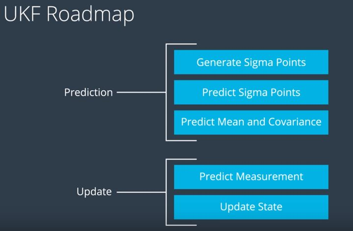
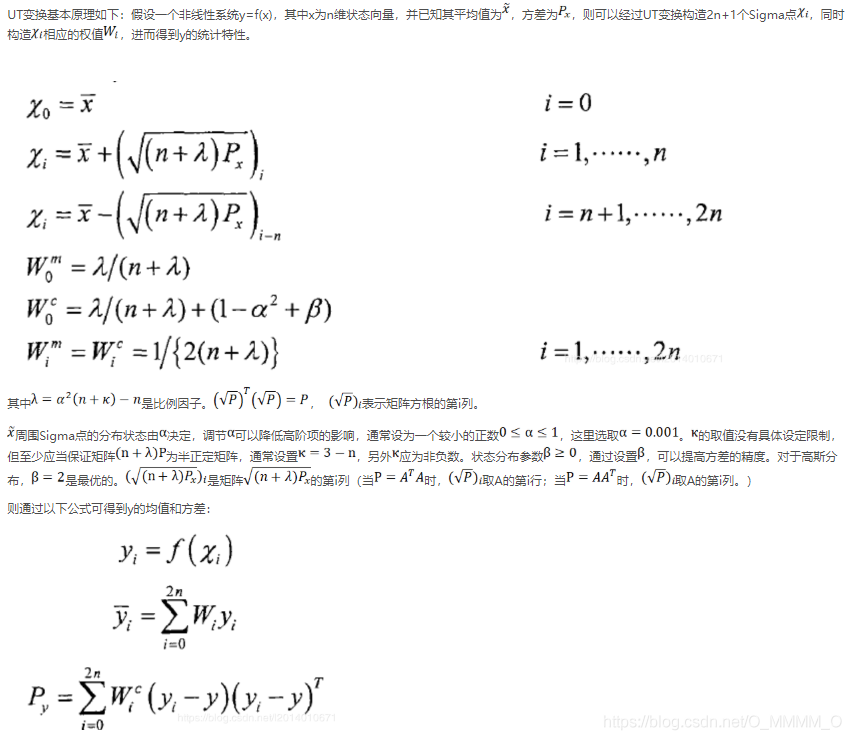
UT变换

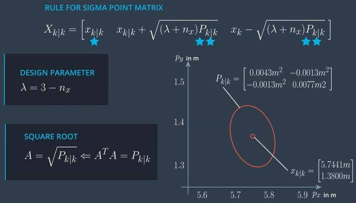
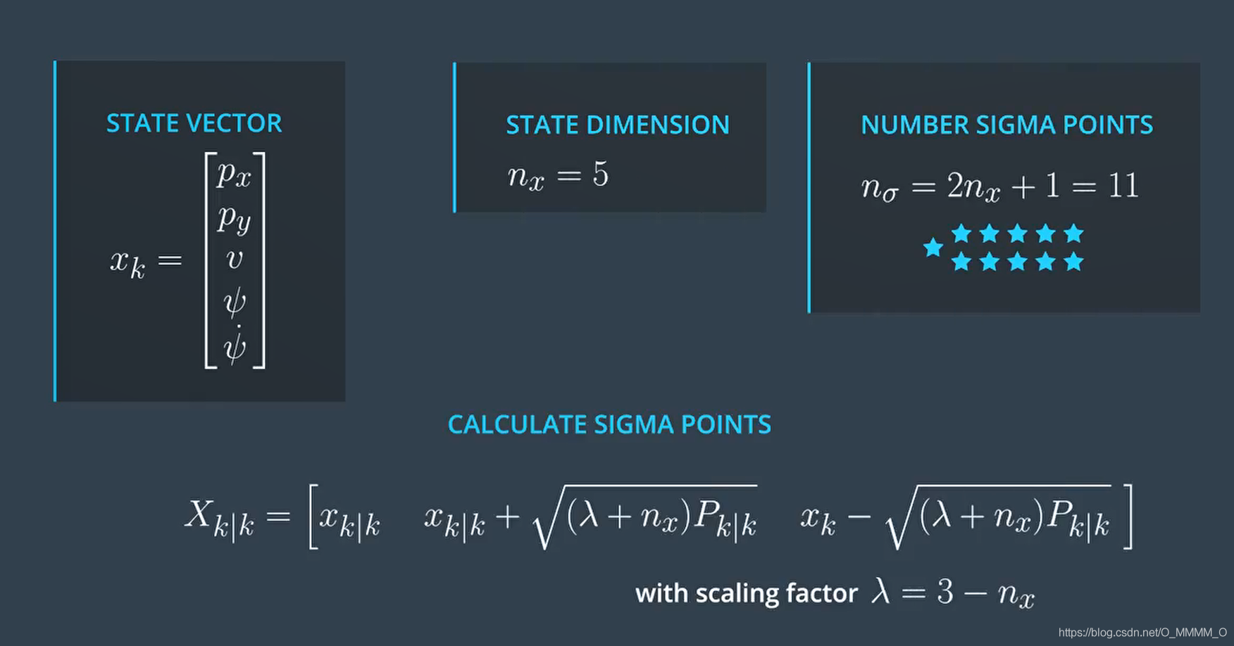
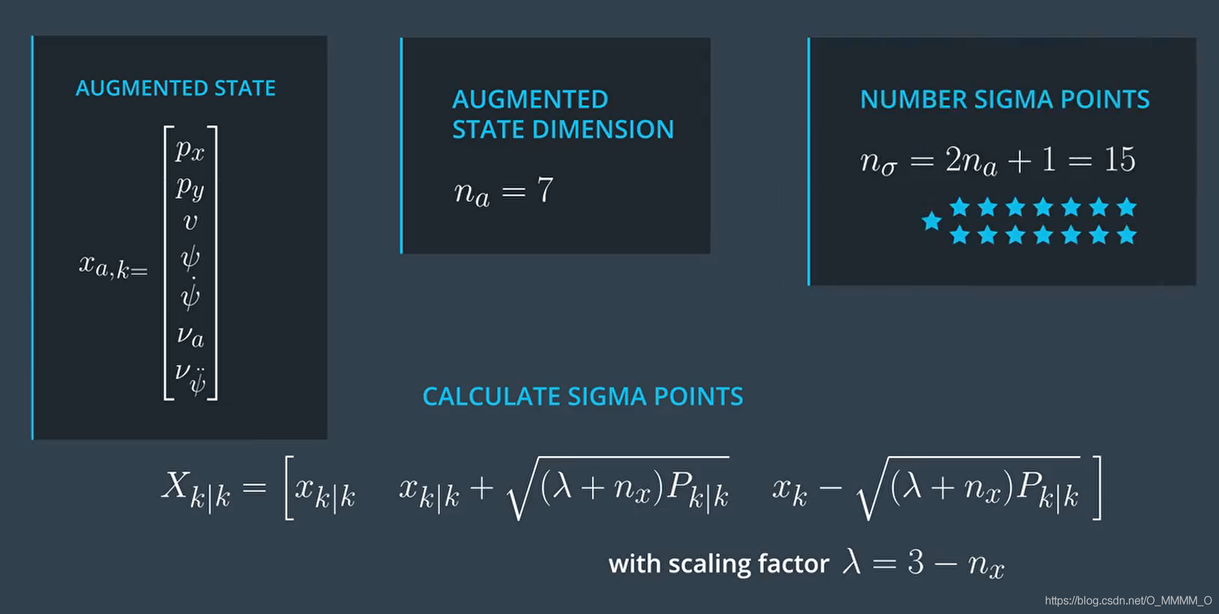
Generate Sigma Points

• 我们的状态向量维度为 $n=5$，Sigma点数为 $2n+1 = 11$
• 每个Sigma Point的协方差矩阵P维度为 5x5
• 所有的Sigma点就组成了 5x11 的矩阵，代表的含义就是按照一定规律生成了环绕在 x 周边的10个点，由这10个点的平均值定义 x 的实际值
• $\lambda$ 是Sigma点离 x 的距离

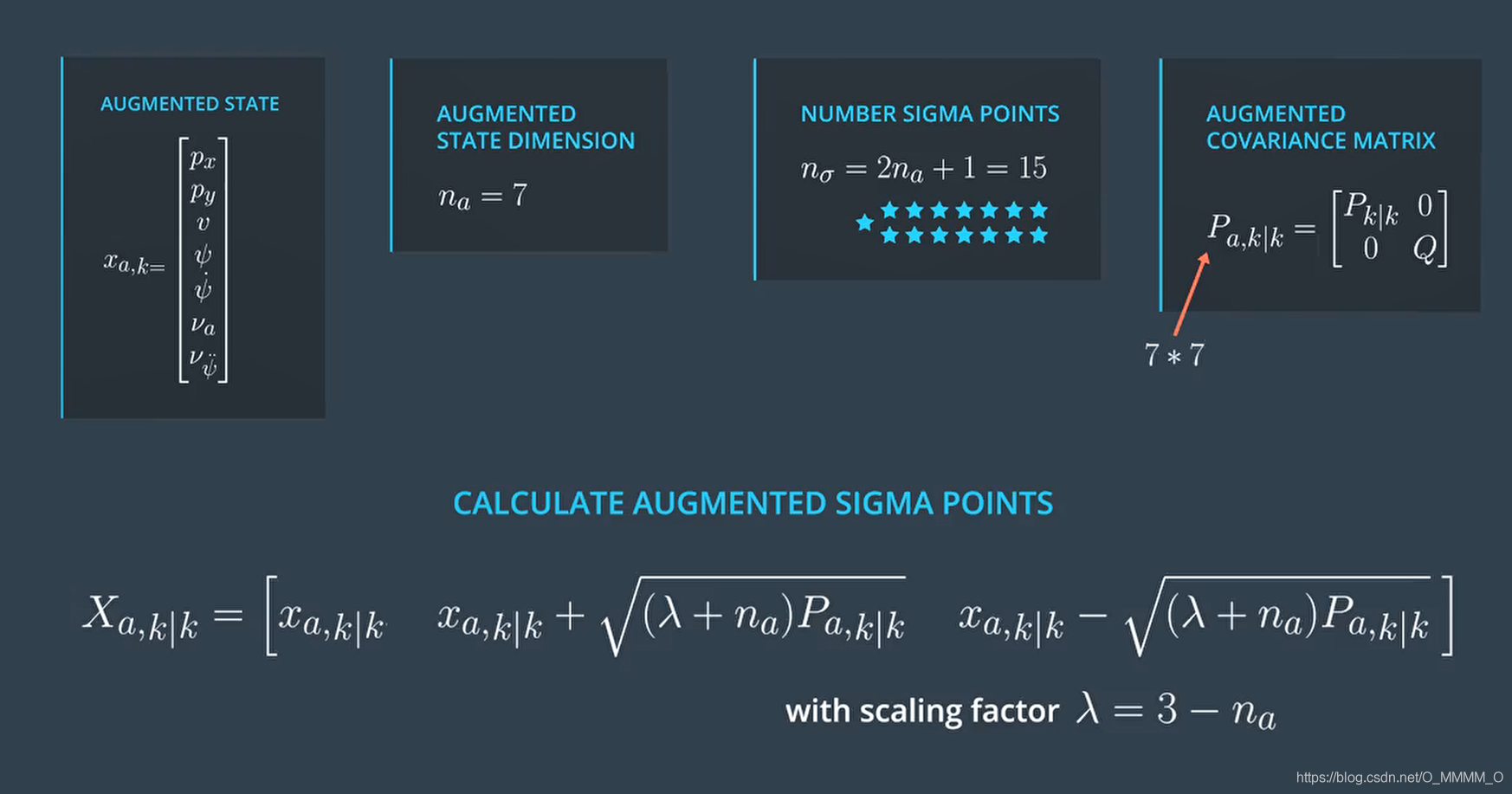
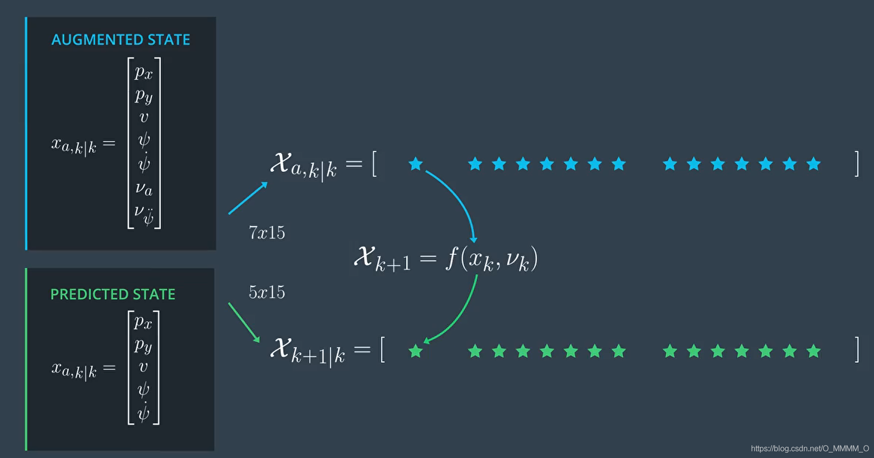
Augmented State (Sigma Points)

考虑到 预测（过程）噪声（加速度与角加速度）

$$\begin{aligned}\nu_{a, k} & \sim N\left(0, \sigma_{a}^{2}\right) \\\nu_{\ddot{\psi}, k} & \sim N\left(0, \sigma_{\ddot{\psi}}^{2}\right)\end{aligned}$$

我们的状态方程里面是有噪声 $v_k$ 的，当这个 $v_k$ 对我们的状态转移矩阵有影响的话，我们需要讲这个噪声考虑到我们的状态转移矩阵里面的，所以我们同时也把 $v_k$ 当作一种状态（噪声状态）放进我们的状态变量空间里。

• 状态向量 augmented_x 维度为 $n=7$，Sigma点数为 $2n+1 = 15$
• 每个Sigma Point的协方差矩阵P augmented_P 维度为 7x7

MatrixXd StatePredictor::compute_augmented_sigma(
  const VectorXd& current_x, const MatrixXd& current_P) {

  MatrixXd augmented_sigma = MatrixXd::Zero(NAUGMENTED, NSIGMA);  // 7 x 15
  VectorXd augmented_x = VectorXd::Zero(NAUGMENTED);              // 7
  MatrixXd augmented_P = MatrixXd::Zero(NAUGMENTED, NAUGMENTED);  // 7 x 7

  augmented_x.head(NX) = current_x;               // 5
  augmented_P.topLeftCorner(NX, NX) = current_P;  // 5 x 5
  augmented_P(NX, NX) = VAR_SPEED_NOISE;
  augmented_P(NX + 1, NX + 1) = VAR_YAWRATE_NOISE;

  const MatrixXd L = augmented_P.llt().matrixL();
  augmented_sigma.col(0) = augmented_x;
  for (int c = 0; c < NAUGMENTED; c++) {
    const int i = c + 1;
    augmented_sigma.col(i) = augmented_x + SCALE * L.col(c);
    augmented_sigma.col(i + NAUGMENTED) = augmented_x - SCALE * L.col(c);
  }

  return augmented_sigma;
}

Predict Process

this->sigma = predict_sigma(augmented_sigma, dt);  // 5 x 15
this->x = predict_x(this->sigma);                  // 5
this->P = predict_P(this->sigma, this->x);         // 5 x 5

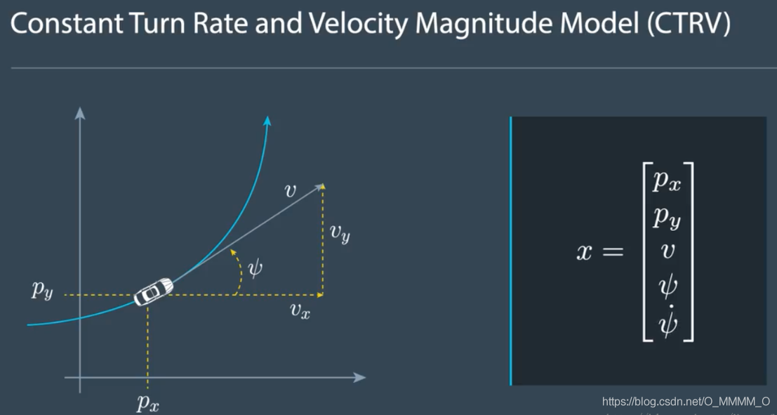
Motion Model (CTRV)

CTRV (constant turn rate and velocity magnitude)

• constant turn rate $\psi$ and velocity $\nu$
• state vector: $n=5$

$$x_{k+1}=x_{k}+\left[\begin{array}{c}\frac{v_{k}}{\dot{\psi}_{k}}\left(\sin \left(\psi_{k}+\dot{\psi}_{k} \Delta t\right)-\sin \left(\psi_{k}\right)\right) \\\frac{v_{k}}{\dot{\psi}_{k}}\left(-\cos \left(\psi_{k}+\dot{\psi_{k}} \Delta t\right)+\cos \left(\psi_{k}\right)\right) \\0 \\\dot{\psi_{k}} \Delta t \\0\end{array}\right] \in \mathbb{R}^5$$

考虑到 过程噪声，该过程模型为

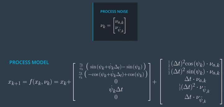
$$x_{k+1}=x_{k}+\left[\begin{array}{c}\frac{v_{k}}{\dot{\psi}_{k}}\left(\sin \left(\psi_{k}+\dot{\psi}_{k} \Delta t\right)-\sin \left(\psi_{k}\right)\right) \\\frac{v_{k}}{\dot{\psi}_{k}}\left(-\cos \left(\psi_{k}+\dot{\psi_{k}} \Delta t\right)+\cos \left(\psi_{k}\right)\right) \\0 \\\dot{\psi_{k}} \Delta t \\0\end{array}\right] + \left[\begin{array}{c} \frac{1}{2} \nu_{a, k} \cos \left(\psi_{k}\right) \Delta t^{2} \\ \frac{1}{2} \nu_{a, k} \sin \left(\psi_{k}\right) \Delta t^{2} \\ \nu_{a, k} \Delta t \\ \frac{1}{2} \nu_{\ddot{\psi}, k} \Delta t^{2} \\ \nu_{\ddot{\psi}, k} \Delta t \end{array}\right] \in \mathbb{R}^5$$

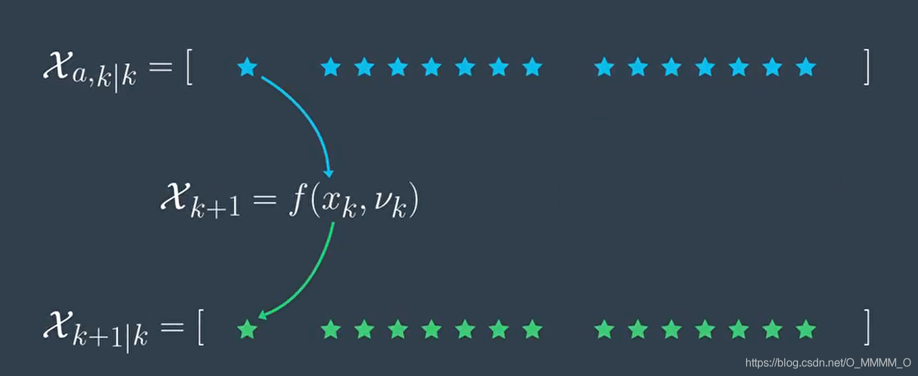
Predict Sigma Points

通过 过程模型，将 增广状态Sigma Points 转换为 预测状态Sigma Points

Predict Mean and Covariance

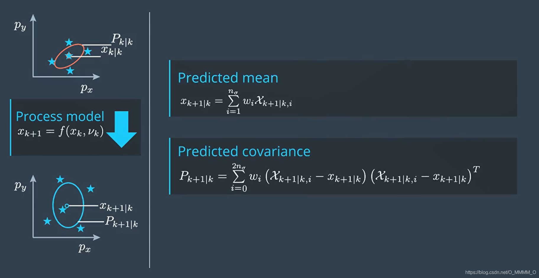
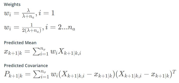
• predicted x

  for (int c = 0; c < NSIGMA; c++) {
    predicted_x += WEIGHTS[c] * predicted_sigma.col(c);
  }

• predicted P

  for (int c = 0; c < NSIGMA; c++) {
    dx = predicted_sigma.col(c) - predicted_x;
    dx(3) = normalize(dx(3));
    predicted_P += WEIGHTS[c] * dx * dx.transpose();
  }

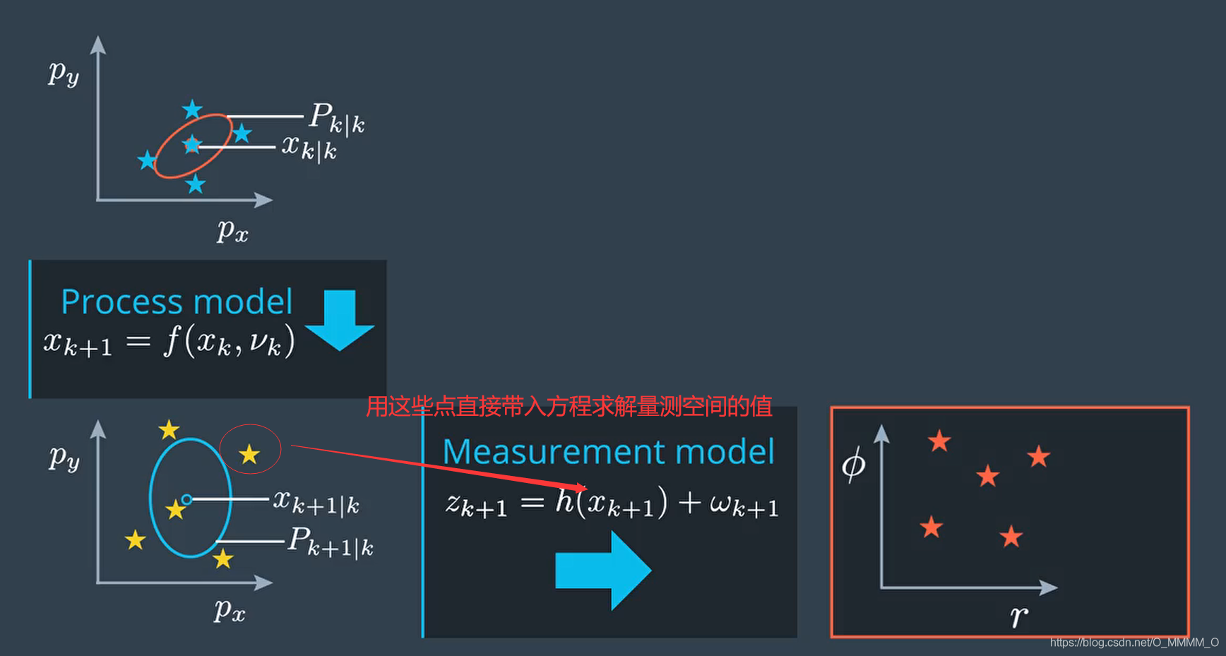
Predict Measurement

针对不同的传感器，测量值z求均值和方差的方式也不同，本文以CTRV模型为基础，通过激光雷达（Lidar）和毫米波雷达（Radar）跟踪车辆位置为例讲解。

this->sigma_z = this->compute_sigma_z(sigma_x);     // 3 x 15 or 2 x 15
this->z = this->compute_z(this->sigma_z);           // 3 or 2
this->S = this->compute_S(this->sigma_z, this->z);  // 3 x 3 or 2 x 2

Lidar测量方程

$$z = \left(\begin{array}{c}{p_{x}} \\ {p_{y}}\end{array}\right)$$

Radar测量方程

$$z = \left(\begin{array}{l} {\rho} \\ {\varphi} \\ {\dot{\rho}} \end{array}\right) = h(x^{\prime}) = \left(\begin{array}{c} {\sqrt{p_{x}^{\prime 2}+p_{y}^{\prime 2}}} \\ {\arctan \left(p_{y}^{\prime} / p_{x}^{\prime}\right)} \\ {\frac{p_{x}^{\prime} v_{x}^{\prime}+p_{y} v_{y}^{\prime}}{\sqrt{p_{x}^{\prime 2}+p_{y}^{\prime 2}}}} \end{array}\right)$$

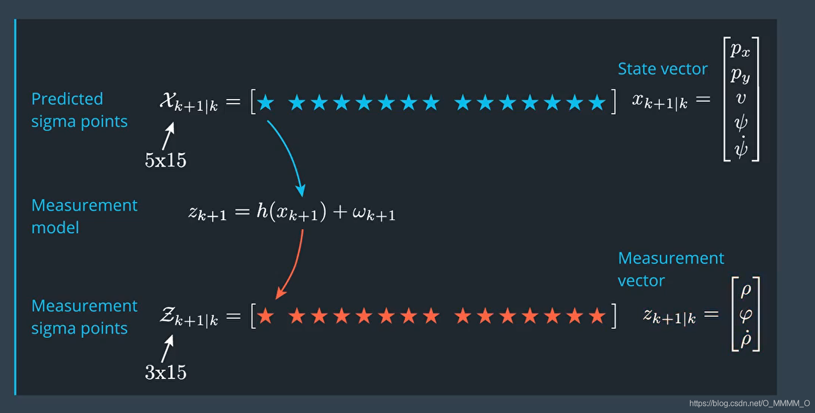
Predict Measurement Sigma Points

• LiDAR Measurement Sigma Points (2 x 15)

• Radar Measurement Sigma Points (3 x 15)

  

for (int c = 0; c < NSIGMA; c++) {
  if (this->current_type == DataPointType::RADAR) {
    const double px = sigma_x(0, c);
    const double py = sigma_x(1, c);
    const double v = sigma_x(2, c);
    const double yaw = sigma_x(3, c);

    const double vx = cos(yaw) * v;
    const double vy = sin(yaw) * v;

    const double rho = sqrt(px * px + py * py);
    const double phi = atan2(py, px);
    const double rhodot = (rho > THRESH) ? ((px * vx + py * vy) / rho) : 0.0;

    sigma(0, c) = rho;
    sigma(1, c) = phi;
    sigma(2, c) = rhodot;

  } else if (this->current_type == DataPointType::LIDAR) {
    sigma(0, c) = sigma_x(0, c);  // px
    sigma(1, c) = sigma_x(1, c);  // py
  }
}

Predict Measurement Mean and Covariance

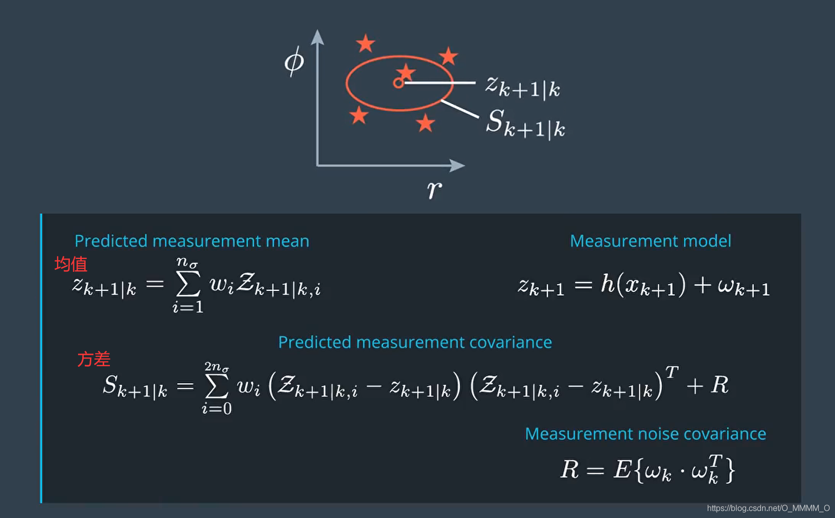
• Predict Measurement Mean

  VectorXd z = VectorXd::Zero(this->nz);
  for (int c = 0; c < NSIGMA; c++) {
    z += WEIGHTS[c] * sigma.col(c);
  }

• Predict Measurement Covariance

  MatrixXd S = MatrixXd::Zero(this->nz, this->nz);
  for (int c = 0; c < NSIGMA; c++) {
    dz = sigma.col(c) - z;
    if (this->current_type == DataPointType::RADAR) {
      dz(1) = normalize(dz(1));
    }
    S += WEIGHTS[c] * dz * dz.transpose();
  }
  S += this->R;

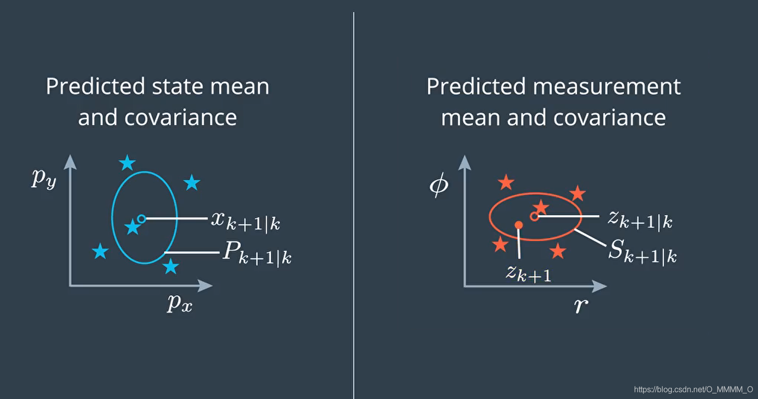
Update State

求出测量值z的均值和方差，然后这两个分布相乘就可以求出新的状态分布了，这个和传统的卡尔曼滤波基本是一样的。

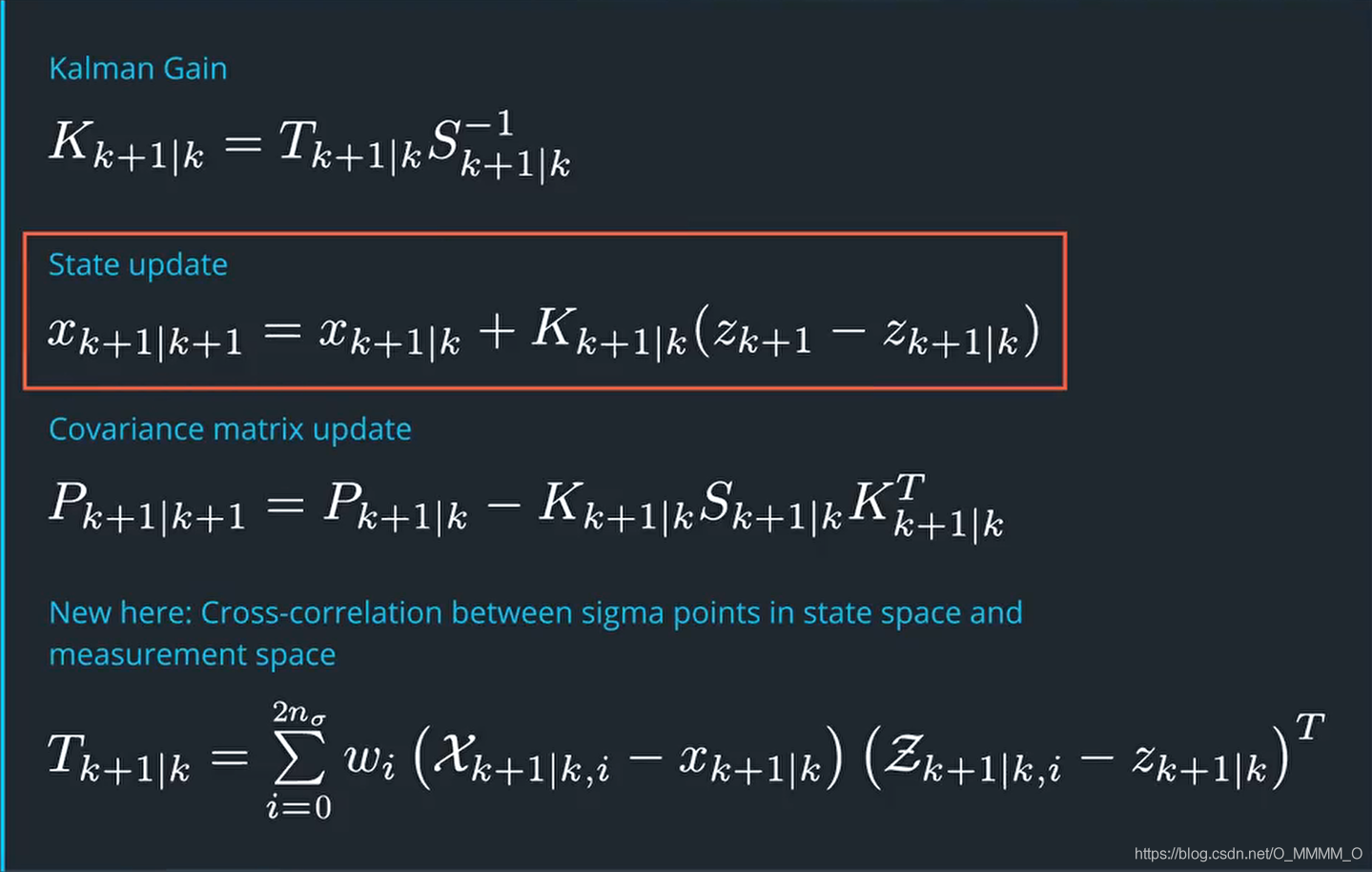
• compute T cross-correlation function，等价于 EKF 中的 $PH^T$

  MatrixXd StateUpdater::compute_Tc(
    const VectorXd& predicted_x, const VectorXd& predicted_z, 
    const MatrixXd& sigma_x, const MatrixXd& sigma_z) {
    
    int NZ = predicted_z.size();
    VectorXd dz;
    VectorXd dx;
    MatrixXd Tc = MatrixXd::Zero(NX, NZ);
  
    for (int c = 0; c < NSIGMA; c++) {
      dx = sigma_x.col(c) - predicted_x;
      dx(3) = normalize(dx(3));
  
      dz = sigma_z.col(c) - predicted_z;
      if (NZ == NZ_RADAR) dz(1) = normalize(dz(1));
  
      Tc += WEIGHTS[c] * dx * dz.transpose();
    }
  
    return Tc;
  }

• update，等价于 EKF更新

  MatrixXd K = Tc * S.inverse();
  
  VectorXd dz = z - predicted_z;
  if (dz.size() == NZ_RADAR) {
    // yaw/phi in radians
    dz(1) = normalize(dz(1));
  }
  
  this->x = predicted_x + K * dz;
  this->P = predicted_P - K * S * K.transpose();

Ref

• 无迹（损）卡尔曼滤波（UKF）理论讲解与实例

• 无人驾驶汽车系统入门（三）——无损卡尔曼滤波，目标追踪，C++

• 学习笔记（优达学城）-无损滤波器 UKF

• Fred159/Udacity-Term2-Project2-UKF